PF: Gravity: Tiled Inversion Linear

Invert data in tiles.

import numpy as np
import matplotlib.pyplot as plt

from discretize import TensorMesh
from SimPEG.potential_fields import gravity
from SimPEG import (
    maps,
    data,
    data_misfit,
    regularization,
    optimization,
    inverse_problem,
    directives,
    inversion,
)
from discretize.utils import mesh_builder_xyz, refine_tree_xyz

try:
    from SimPEG import utils
    from SimPEG.utils import plot2Ddata
except:
    from SimPEG import Utils as utils
    from SimPEG.Utils.Plotutils import plot2Ddata

import shutil

Setup

Define the survey and model parameters

Create an a global survey and mesh and simulate some data

# Create and array of observation points
xr = np.linspace(-30.0, 30.0, 20)
yr = np.linspace(-30.0, 30.0, 20)
X, Y = np.meshgrid(xr, yr)

# Move the observation points 5m above the topo
Z = -np.exp((X ** 2 + Y ** 2) / 75 ** 2)

# Create a topo array
topo = np.c_[utils.mkvc(X.T), utils.mkvc(Y.T), utils.mkvc(Z.T)]

# Create station locations drapped 0.1 m above topo
rxLoc = np.c_[utils.mkvc(X.T), utils.mkvc(Y.T), utils.mkvc(Z.T) + 0.1]

Divided and Conquer

Split the data set in two and create sub-problems

# Mesh parameters
h = [5, 5, 5]
padDist = np.ones((3, 2)) * 100
octree_levels = [8, 4]

# Create tiles
local_indices = [rxLoc[:, 0] <= 0, rxLoc[:, 0] > 0]
local_surveys = []
local_meshes = []
for local_index in local_indices:

    receivers = gravity.receivers.Point(rxLoc[local_index, :])
    srcField = gravity.sources.SourceField([receivers])
    local_survey = gravity.survey.Survey(srcField)

    # Create a local mesh that covers all points, but refined on the local survey
    local_mesh = mesh_builder_xyz(
        topo, h, padding_distance=padDist, depth_core=100, mesh_type="tree"
    )
    local_mesh = refine_tree_xyz(
        local_mesh,
        local_survey.receiver_locations,
        method="surface",
        octree_levels=octree_levels,
        finalize=True,
    )

    local_surveys.append(local_survey)
    local_meshes.append(local_mesh)

Global Mesh

Create a global mesh survey for simulation

mesh = mesh_builder_xyz(
    topo, h, padding_distance=padDist, depth_core=100, mesh_type="tree"
)

# This garantees that the local meshes are always coarser or equal
for local_mesh in local_meshes:
    mesh.insert_cells(
        local_mesh.gridCC,
        local_mesh.cell_levels_by_index(np.arange(local_mesh.nC)),
        finalize=False,
    )
mesh.finalize()

# Define an active cells from topo
activeCells = utils.surface2ind_topo(mesh, topo)
nC = int(activeCells.sum())

# We can now create a density model and generate data
# Here a simple block in half-space
# Get the indicies of the magnetized block
model = np.zeros(mesh.nC)
ind = utils.ModelBuilder.getIndicesBlock(
    np.r_[-10, -10, -30], np.r_[10, 10, -10], mesh.gridCC,
)[0]

# Assign magnetization values
model[ind] = 0.3

# Remove air cells
model = model[activeCells]

# Create reduced identity map
idenMap = maps.IdentityMap(nP=nC)

# Create a global survey just for simulation of data
receivers = gravity.receivers.Point(rxLoc)
srcField = gravity.sources.SourceField([receivers])
survey = gravity.survey.Survey(srcField)

# Create the forward simulation for the global dataset
simulation = gravity.simulation.Simulation3DIntegral(
    survey=survey, mesh=mesh, rhoMap=idenMap, actInd=activeCells
)

# Compute linear forward operator and compute some data
d = simulation.fields(model)

# Add noise and uncertainties
# We add some random Gaussian noise (1nT)
synthetic_data = d + np.random.randn(len(d)) * 1e-3
wd = np.ones(len(synthetic_data)) * 1e-3  # Assign flat uncertainties

Tiled misfits

local_misfits = []
for ii, local_survey in enumerate(local_surveys):

    tile_map = maps.TileMap(mesh, activeCells, local_meshes[ii])

    local_actives = tile_map.local_active

    # Create the forward simulation
    simulation = gravity.simulation.Simulation3DIntegral(
        survey=local_survey,
        mesh=local_meshes[ii],
        rhoMap=tile_map,
        actInd=local_actives,
        sensitivity_path=f"Inversion\Tile{ii}.zarr",
    )

    data_object = data.Data(
        local_survey,
        dobs=synthetic_data[local_indices[ii]],
        standard_deviation=wd[local_indices[ii]],
    )

    local_misfits.append(
        data_misfit.L2DataMisfit(data=data_object, simulation=simulation)
    )


# Our global misfit
global_misfit = local_misfits[0] + local_misfits[1]

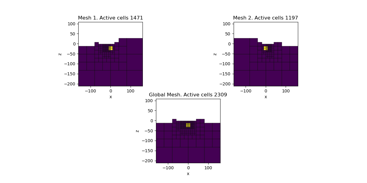
# Plot the model on different meshes
fig = plt.figure(figsize=(12, 6))
for ii, local_misfit in enumerate(local_misfits):

    local_mesh = local_misfit.simulation.mesh
    local_map = local_misfit.simulation.rhoMap

    inject_local = maps.InjectActiveCells(local_mesh, local_map.local_active, np.nan)

    ax = plt.subplot(2, 2, ii + 1)
    local_mesh.plotSlice(
        inject_local * (local_map * model), normal="Y", ax=ax, grid=True
    )
    ax.set_aspect("equal")
    ax.set_title(f"Mesh {ii+1}. Active cells {local_map.local_active.sum()}")


# Create active map to go from reduce set to full
inject_global = maps.InjectActiveCells(mesh, activeCells, np.nan)

ax = plt.subplot(2, 1, 2)
mesh.plotSlice(inject_global * model, normal="Y", ax=ax, grid=True)
ax.set_title(f"Global Mesh. Active cells {activeCells.sum()}")
ax.set_aspect("equal")
plt.show()

Out:

/Users/josephcapriotti/codes/simpeg/examples/02-gravity/plot_inv_grav_tiled.py:217: UserWarning: Matplotlib is currently using agg, which is a non-GUI backend, so cannot show the figure.
  plt.show()

Invert on the global mesh

# Create reduced identity map
idenMap = maps.IdentityMap(nP=nC)

# Create a regularization
reg = regularization.Sparse(mesh, indActive=activeCells, mapping=idenMap)

m0 = np.ones(nC) * 1e-4  # Starting model

# Add directives to the inversion
opt = optimization.ProjectedGNCG(
    maxIter=100, lower=-1.0, upper=1.0, maxIterLS=20, maxIterCG=10, tolCG=1e-3
)
invProb = inverse_problem.BaseInvProblem(global_misfit, reg, opt)
betaest = directives.BetaEstimate_ByEig(beta0_ratio=1e-1)

# Here is where the norms are applied
# Use pick a threshold parameter empirically based on the distribution of
# model parameters
update_IRLS = directives.Update_IRLS(
    f_min_change=1e-4, max_irls_iterations=0, coolEpsFact=1.5, beta_tol=1e-2,
)
saveDict = directives.SaveOutputEveryIteration(save_txt=False)
update_Jacobi = directives.UpdatePreconditioner()
sensitivity_weights = directives.UpdateSensitivityWeights(everyIter=False)
inv = inversion.BaseInversion(
    invProb,
    directiveList=[update_IRLS, sensitivity_weights, betaest, update_Jacobi, saveDict],
)

# Run the inversion
mrec = inv.run(m0)


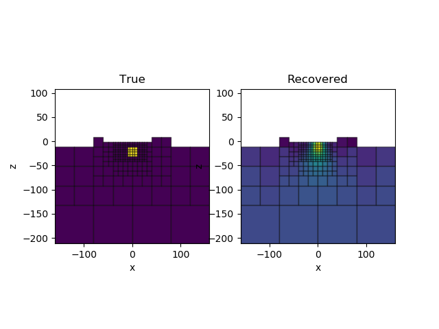
# Plot the result
ax = plt.subplot(1, 2, 1)
mesh.plotSlice(inject_global * model, normal="Y", ax=ax, grid=True)
ax.set_title("True")
ax.set_aspect("equal")

ax = plt.subplot(1, 2, 2)
mesh.plotSlice(inject_global * mrec, normal="Y", ax=ax, grid=True)
ax.set_title("Recovered")
ax.set_aspect("equal")
plt.show()

Out:

SimPEG.InvProblem will set Regularization.mref to m0.

        SimPEG.InvProblem is setting bfgsH0 to the inverse of the eval2Deriv.
        ***Done using same Solver and solver_opts as the Simulation3DIntegral problem***
model has any nan: 0
=============================== Projected GNCG ===============================
  #     beta     phi_d     phi_m       f      |proj(x-g)-x|  LS    Comment
-----------------------------------------------------------------------------
x0 has any nan: 0
   0  3.49e+06  4.21e+04  0.00e+00  4.21e+04    4.80e+01      0
   1  1.75e+06  4.42e+03  1.07e-03  6.29e+03    4.77e+01      0
   2  8.73e+05  2.36e+03  1.91e-03  4.02e+03    4.74e+01      0   Skip BFGS
   3  4.37e+05  1.12e+03  2.89e-03  2.38e+03    4.72e+01      0   Skip BFGS
   4  2.18e+05  5.34e+02  3.82e-03  1.37e+03    4.67e+01      0   Skip BFGS
   5  1.09e+05  2.90e+02  4.58e-03  7.90e+02    4.61e+01      0   Skip BFGS
Reached starting chifact with l2-norm regularization: Start IRLS steps...
eps_p: 0.07141989320928005 eps_q: 0.07141989320928005
Reach maximum number of IRLS cycles: 0
------------------------- STOP! -------------------------
1 : |fc-fOld| = 0.0000e+00 <= tolF*(1+|f0|) = 4.2128e+03
1 : |xc-x_last| = 3.8487e-02 <= tolX*(1+|x0|) = 1.0048e-01
0 : |proj(x-g)-x|    = 4.6036e+01 <= tolG          = 1.0000e-01
0 : |proj(x-g)-x|    = 4.6036e+01 <= 1e3*eps       = 1.0000e-02
0 : maxIter   =     100    <= iter          =      6
------------------------- DONE! -------------------------
/Users/josephcapriotti/codes/simpeg/examples/02-gravity/plot_inv_grav_tiled.py:271: UserWarning: Matplotlib is currently using agg, which is a non-GUI backend, so cannot show the figure.
  plt.show()