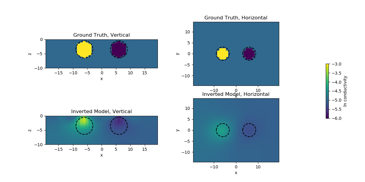
3D DC inversion of Dipole Dipole array

This is an example for 3D DC inversion. The model consists of 2 spheres, one conductive, the other one resistive compared to the background.

We restrain the inversion to the Core Mesh through the use an Active Cells mapping that we combine with an exponetial mapping to invert in log conductivity space. Here mapping, \(\mathcal{M}\), indicates transformation of our model to a different space:

\[\sigma = \mathcal{M}(\mathbf{m})\]

Following example will show you how user can implement a 3D DC inversion.

import discretize
from SimPEG import (
    maps,
    utils,
    data_misfit,
    regularization,
    optimization,
    inverse_problem,
    directives,
    inversion,
)
from SimPEG.electromagnetics.static import resistivity as DC, utils as DCutils
import numpy as np
import matplotlib.pyplot as plt

try:
    from pymatsolver import Pardiso as Solver
except ImportError:
    from SimPEG import SolverLU as Solver

np.random.seed(12345)

# 3D Mesh
#########

# Cell sizes
csx, csy, csz = 1.0, 1.0, 0.5
# Number of core cells in each direction
ncx, ncy, ncz = 41, 31, 21
# Number of padding cells to add in each direction
npad = 7
# Vectors of cell lengths in each direction with padding
hx = [(csx, npad, -1.5), (csx, ncx), (csx, npad, 1.5)]
hy = [(csy, npad, -1.5), (csy, ncy), (csy, npad, 1.5)]
hz = [(csz, npad, -1.5), (csz, ncz)]
# Create mesh and center it
mesh = discretize.TensorMesh([hx, hy, hz], x0="CCN")

# 2-spheres Model Creation

# Spheres parameters
x0, y0, z0, r0 = -6.0, 0.0, -3.5, 3.0
x1, y1, z1, r1 = 6.0, 0.0, -3.5, 3.0

# ln conductivity
ln_sigback = -5.0
ln_sigc = -3.0
ln_sigr = -6.0

# Define model
# Background
mtrue = ln_sigback * np.ones(mesh.nC)

# Conductive sphere
csph = (
    np.sqrt(
        (mesh.gridCC[:, 0] - x0) ** 2.0
        + (mesh.gridCC[:, 1] - y0) ** 2.0
        + (mesh.gridCC[:, 2] - z0) ** 2.0
    )
) < r0
mtrue[csph] = ln_sigc * np.ones_like(mtrue[csph])

# Resistive Sphere
rsph = (
    np.sqrt(
        (mesh.gridCC[:, 0] - x1) ** 2.0
        + (mesh.gridCC[:, 1] - y1) ** 2.0
        + (mesh.gridCC[:, 2] - z1) ** 2.0
    )
) < r1
mtrue[rsph] = ln_sigr * np.ones_like(mtrue[rsph])

# Extract Core Mesh
xmin, xmax = -20.0, 20.0
ymin, ymax = -15.0, 15.0
zmin, zmax = -10.0, 0.0
xyzlim = np.r_[[[xmin, xmax], [ymin, ymax], [zmin, zmax]]]
actind, meshCore = utils.mesh_utils.ExtractCoreMesh(xyzlim, mesh)


# Function to plot cylinder border
def getCylinderPoints(xc, zc, r):
    xLocOrig1 = np.arange(-r, r + r / 10.0, r / 10.0)
    xLocOrig2 = np.arange(r, -r - r / 10.0, -r / 10.0)
    # Top half of cylinder
    zLoc1 = np.sqrt(-(xLocOrig1 ** 2.0) + r ** 2.0) + zc
    # Bottom half of cylinder
    zLoc2 = -np.sqrt(-(xLocOrig2 ** 2.0) + r ** 2.0) + zc
    # Shift from x = 0 to xc
    xLoc1 = xLocOrig1 + xc * np.ones_like(xLocOrig1)
    xLoc2 = xLocOrig2 + xc * np.ones_like(xLocOrig2)

    topHalf = np.vstack([xLoc1, zLoc1]).T
    topHalf = topHalf[0:-1, :]
    bottomHalf = np.vstack([xLoc2, zLoc2]).T
    bottomHalf = bottomHalf[0:-1, :]

    cylinderPoints = np.vstack([topHalf, bottomHalf])
    cylinderPoints = np.vstack([cylinderPoints, topHalf[0, :]])
    return cylinderPoints


# Setup a synthetic Dipole-Dipole Survey
# Line 1
xmin, xmax = -15.0, 15.0
ymin, ymax = 0.0, 0.0
zmin, zmax = 0, 0
endl = np.array([[xmin, ymin, zmin], [xmax, ymax, zmax]])
survey1 = DCutils.gen_DCIPsurvey(endl, "dipole-dipole", dim=mesh.dim, a=3, b=3, n=8)

# Line 2
xmin, xmax = -15.0, 15.0
ymin, ymax = 5.0, 5.0
zmin, zmax = 0, 0
endl = np.array([[xmin, ymin, zmin], [xmax, ymax, zmax]])
survey2 = DCutils.gen_DCIPsurvey(endl, "dipole-dipole", dim=mesh.dim, a=3, b=3, n=8)

# Line 3
xmin, xmax = -15.0, 15.0
ymin, ymax = -5.0, -5.0
zmin, zmax = 0, 0
endl = np.array([[xmin, ymin, zmin], [xmax, ymax, zmax]])
survey3 = DCutils.gen_DCIPsurvey(endl, "dipole-dipole", dim=mesh.dim, a=3, b=3, n=8)

# Concatenate lines
survey = DC.Survey(survey1.source_list + survey2.source_list + survey3.source_list)

# Setup Problem with exponential mapping and Active cells only in the core mesh
expmap = maps.ExpMap(mesh)
mapactive = maps.InjectActiveCells(mesh=mesh, indActive=actind, valInactive=-5.0)
mapping = expmap * mapactive
problem = DC.Simulation3DCellCentered(
    mesh, survey=survey, sigmaMap=mapping, solver=Solver, bc_type="Neumann"
)

data = problem.make_synthetic_data(mtrue[actind], relative_error=0.05, add_noise=True)

# Tikhonov Inversion

# Initial Model
m0 = np.median(ln_sigback) * np.ones(mapping.nP)
# Data Misfit
dmis = data_misfit.L2DataMisfit(simulation=problem, data=data)
# Regularization
regT = regularization.Simple(
    mesh, indActive=actind, alpha_s=1e-6, alpha_x=1.0, alpha_y=1.0, alpha_z=1.0
)

# Optimization Scheme
opt = optimization.InexactGaussNewton(maxIter=10)

# Form the problem
opt.remember("xc")
invProb = inverse_problem.BaseInvProblem(dmis, regT, opt)

# Directives for Inversions
beta = directives.BetaEstimate_ByEig(beta0_ratio=1e1)
Target = directives.TargetMisfit()
betaSched = directives.BetaSchedule(coolingFactor=5.0, coolingRate=2)

inv = inversion.BaseInversion(invProb, directiveList=[beta, Target, betaSched])
# Run Inversion
minv = inv.run(m0)

# Final Plot
############

fig, ax = plt.subplots(2, 2, figsize=(12, 6))
ax = utils.mkvc(ax)

cyl0v = getCylinderPoints(x0, z0, r0)
cyl1v = getCylinderPoints(x1, z1, r1)

cyl0h = getCylinderPoints(x0, y0, r0)
cyl1h = getCylinderPoints(x1, y1, r1)

clim = [(mtrue[actind]).min(), (mtrue[actind]).max()]

dat = meshCore.plotSlice(
    ((mtrue[actind])), ax=ax[0], normal="Y", clim=clim, ind=int(ncy / 2)
)
ax[0].set_title("Ground Truth, Vertical")
ax[0].set_aspect("equal")

meshCore.plotSlice((minv), ax=ax[1], normal="Y", clim=clim, ind=int(ncy / 2))
ax[1].set_aspect("equal")
ax[1].set_title("Inverted Model, Vertical")

meshCore.plotSlice(((mtrue[actind])), ax=ax[2], normal="Z", clim=clim, ind=int(ncz / 2))
ax[2].set_title("Ground Truth, Horizontal")
ax[2].set_aspect("equal")

meshCore.plotSlice((minv), ax=ax[3], normal="Z", clim=clim, ind=int(ncz / 2))
ax[3].set_title("Inverted Model, Horizontal")
ax[3].set_aspect("equal")

for i in range(2):
    ax[i].plot(cyl0v[:, 0], cyl0v[:, 1], "k--")
    ax[i].plot(cyl1v[:, 0], cyl1v[:, 1], "k--")
for i in range(2, 4):
    ax[i].plot(cyl1h[:, 0], cyl1h[:, 1], "k--")
    ax[i].plot(cyl0h[:, 0], cyl0h[:, 1], "k--")

fig.subplots_adjust(right=0.8)
cbar_ax = fig.add_axes([0.85, 0.15, 0.05, 0.7])
cb = plt.colorbar(dat[0], ax=cbar_ax)
cb.set_label("ln conductivity")

cbar_ax.axis("off")

plt.show()

Out:

SimPEG.InvProblem will set Regularization.mref to m0.

        SimPEG.InvProblem is setting bfgsH0 to the inverse of the eval2Deriv.
        ***Done using same Solver and solverOpts as the problem***
model has any nan: 0
============================ Inexact Gauss Newton ============================
  #     beta     phi_d     phi_m       f      |proj(x-g)-x|  LS    Comment
-----------------------------------------------------------------------------
x0 has any nan: 0
   0  2.66e+01  2.54e+03  0.00e+00  2.54e+03    5.66e+02      0
   1  2.66e+01  3.45e+02  5.89e+00  5.02e+02    5.93e+01      0
   2  5.31e+00  2.30e+02  8.55e+00  2.75e+02    4.65e+01      0   Skip BFGS
   3  5.31e+00  9.17e+01  1.90e+01  1.93e+02    1.74e+01      0
   4  1.06e+00  7.42e+01  2.05e+01  9.60e+01    1.94e+01      0
------------------------- STOP! -------------------------
1 : |fc-fOld| = 0.0000e+00 <= tolF*(1+|f0|) = 2.5374e+02
1 : |xc-x_last| = 3.8956e+00 <= tolX*(1+|x0|) = 7.5300e+01
0 : |proj(x-g)-x|    = 1.9387e+01 <= tolG          = 1.0000e-01
0 : |proj(x-g)-x|    = 1.9387e+01 <= 1e3*eps       = 1.0000e-02
0 : maxIter   =      10    <= iter          =      5
------------------------- DONE! -------------------------
/Users/josephcapriotti/codes/simpeg/examples/04-dcip/plot_inv_dcip_dipoledipole_3Dinversion_twospheres.py:232: UserWarning: Matplotlib is currently using agg, which is a non-GUI backend, so cannot show the figure.
  plt.show()