Time-domain CSEM for a resistive cube in a deep marine setting

import empymod
import discretize
import pymatsolver
import numpy as np
import SimPEG
from SimPEG import maps
from SimPEG.electromagnetics import time_domain as TDEM
import matplotlib.pyplot as plt

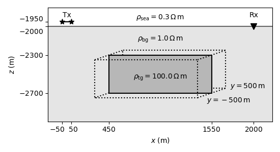
(A) Model

fig = plt.figure(figsize=(5.5, 3))
ax = plt.gca()

# Seafloor and background
plt.plot([-200, 2200], [-2000, -2000], "-", c=".4")
bg = plt.Rectangle((-500, -3000), 3000, 1000, facecolor="black", alpha=0.1)
ax.add_patch(bg)

# Plot survey
plt.plot([-50, 50], [-1950, -1950], "*-", ms=8, c="k")
plt.plot(2000, -2000, "v", ms=8, c="k")
plt.text(0, -1900, r"Tx", horizontalalignment="center")
plt.text(2000, -1900, r"Rx", horizontalalignment="center")

# Plot cube
plt.plot([450, 1550, 1550, 450, 450], [-2300, -2300, -2700, -2700, -2300], "k-")
plt.plot([300, 1400, 1400, 300, 300], [-2350, -2350, -2750, -2750, -2350], "k:")
plt.plot([600, 600, 1700, 1700, 1550], [-2300, -2250, -2250, -2650, -2650], "k:")
plt.plot([300, 600], [-2350, -2250], "k:")
plt.plot([1400, 1700], [-2350, -2250], "k:")
plt.plot([300, 450], [-2750, -2700], "k:")
plt.plot([1400, 1700], [-2750, -2650], "k:")
tg = plt.Rectangle((450, -2700), 1100, 400, facecolor="black", alpha=0.2)
ax.add_patch(tg)

# Annotate resistivities
plt.text(
    1000, -1925, r"$\rho_\mathrm{sea}=0.3\,\Omega\,$m", horizontalalignment="center"
)
plt.text(
    1000, -2150, r"$\rho_\mathrm{bg}=1.0\,\Omega\,$m", horizontalalignment="center"
)
plt.text(
    1000, -2550, r"$\rho_\mathrm{tg}=100.0\,\Omega\,$m", horizontalalignment="center"
)
plt.text(1500, -2800, r"$y=-500\,$m", horizontalalignment="left")
plt.text(1750, -2650, r"$y=500\,$m", horizontalalignment="left")

# Ticks and labels
plt.xticks(
    [-50, 50, 450, 1550, 2000],
    ["$-50~$ $~$  $~$", " $~50$", "$450$", "$1550$", "$2000$"],
)
plt.yticks(
    [-1950, -2000, -2300, -2700], ["$-1950$\n", "\n$-2000$", "$-2300$", "$-2700$"]
)

plt.xlim([-200, 2200])
plt.ylim([-3000, -1800])

plt.xlabel("$x$ (m)")
plt.ylabel("$z$ (m)")
plt.tight_layout()

plt.show()

Out:

/Users/josephcapriotti/codes/simpeg/examples/06-tdem/plot_fwd_tdem_3d_model.py:71: UserWarning: Matplotlib is currently using agg, which is a non-GUI backend, so cannot show the figure.
  plt.show()

# Resistivities
res_sea = 0.3
res_bg = 1.0
res_tg = 100.0

# Seafloor
seafloor = -2000

# Target dimension
tg_x = [450, 1550]
tg_y = [-500, 500]
tg_z = [-2700, -2300]

(B) Survey

# Source: 100 m x-directed diplole at the origin,
# 50 m above seafloor, src [x1, x2, y1, y2, z1, z2]
src = [-50, 50, 0, 0, -1950, -1950]

# Receiver: x-directed dipole at 2 km on the
# seafloor, rec = [x, y, z, azimuth, dip]
rec = [2000, 0, -2000, 0, 0]

# Times to compute, 0.1 - 10 s, 301 steps
times = np.logspace(-1, 1, 301)

(C) Modelling parameters

Check diffusion distances

# Get min/max diffusion distances for the two halfspaces.
diff_dist0 = 1261 * np.sqrt(np.r_[times * res_sea, times * res_sea])
diff_dist1 = 1261 * np.sqrt(np.r_[times * res_bg, times * res_bg])
diff_dist2 = 1261 * np.sqrt(np.r_[times * res_tg, times * res_tg])
print("Min/max diffusion distance:")
print(f"- Water      :: {diff_dist0.min():8.0f} / {diff_dist0.max():8.0f} m.")
print(f"- Background :: {diff_dist1.min():8.0f} / {diff_dist1.max():8.0f} m.")
print(f"- Target     :: {diff_dist2.min():8.0f} / {diff_dist2.max():8.0f} m.")

Out:

Min/max diffusion distance:
- Water      ::      218 /     2184 m.
- Background ::      399 /     3988 m.
- Target     ::     3988 /    39876 m.

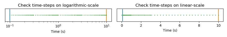
Time-steps

# Time steps
time_steps = [1e-1, (1e-2, 21), (3e-2, 23), (1e-1, 21), (3e-1, 23)]

# Create mesh with time steps
ts = discretize.TensorMesh([time_steps]).vectorNx

# Plot them
plt.figure(figsize=(9, 1.5))

# Logarithmic scale
plt.subplot(121)
plt.title("Check time-steps on logarithmic-scale")
plt.plot([times.min(), times.min()], [-1, 1])
plt.plot([times.max(), times.max()], [-1, 1])
plt.plot(ts, ts * 0, ".", ms=2)
plt.yticks([])
plt.xscale("log")
plt.xlabel("Time (s)")

# Linear scale
plt.subplot(122)
plt.title("Check time-steps on linear-scale")
plt.plot([times.min(), times.min()], [-1, 1])
plt.plot([times.max(), times.max()], [-1, 1])
plt.plot(ts, ts * 0, ".", ms=2)
plt.yticks([])
plt.xlabel("Time (s)")

plt.tight_layout()
plt.show()

# Check times with time-steps
print(f"Min/max times    : {times.min():.1e} / {times.max():.1e}")
print(f"Min/max timeSteps: {ts[1]:.1e} / {ts[-1]:.1e}")

Out:

/Users/josephcapriotti/codes/simpeg/examples/06-tdem/plot_fwd_tdem_3d_model.py:155: UserWarning: Matplotlib is currently using agg, which is a non-GUI backend, so cannot show the figure.
  plt.show()
Min/max times    : 1.0e-01 / 1.0e+01
Min/max timeSteps: 1.0e-01 / 1.0e+01

Create mesh (discretize)

# Cell width, number of cells
width = 100
nx = rec[0] // width + 4
ny = 10
nz = 9

# Padding
npadx = 14
npadyz = 12

# Stretching
alpha = 1.3

# Initiate TensorMesh
mesh = discretize.TensorMesh(
    [
        [(width, npadx, -alpha), (width, nx), (width, npadx, alpha)],
        [(width, npadyz, -alpha), (width, ny), (width, npadyz, alpha)],
        [(width, npadyz, -alpha), (width, nz), (width, npadyz, alpha)],
    ],
    x0="CCC",
)

# Shift mesh so that
# x=0 is at midpoint of source;
# z=-2000 is at receiver level
mesh.x0[0] += rec[0] // 2 - width / 2
mesh.x0[2] -= nz / 2 * width - seafloor
mesh

TensorMesh			58,344 cells
		MESH EXTENT		CELL WIDTH		FACTOR
dir	nC	min	max	min	max	max
x	52	-16,878.63	18,778.63	100.00	3,937.38	1.30
y	34	-10,162.50	10,162.50	100.00	2,329.81	1.30
z	33	-12,562.50	7,662.50	100.00	2,329.81	1.30

Check if source and receiver are exactly at x-edges.

No requirement; if receiver are exactly on x-edges then no interpolation is required to get the responses (cell centers in x, cell edges in y, z).

print(
    f"Rec-{{x;y;z}} :: {rec[0] in np.round(mesh.vectorCCx)!s:>5}; "
    f"{rec[1] in np.round(mesh.vectorNy)!s:>5}; "
    f"{rec[2] in np.round(mesh.vectorNz)!s:>5}"
)
print(
    f"Src-x       :: {src[0] in np.round(mesh.vectorCCx)!s:>5}; "
    f"{src[1] in np.round(mesh.vectorCCx)!s:>5}"
)
print(
    f"Src-y       :: {src[2] in np.round(mesh.vectorNy)!s:>5}; "
    f"{src[3] in np.round(mesh.vectorNy)!s:>5}"
)
print(
    f"Src-z       :: {src[4] in np.round(mesh.vectorNz)!s:>5}; "
    f"{src[5] in np.round(mesh.vectorNz)!s:>5}"
)

Out:

Rec-{x;y;z} ::  True;  True;  True
Src-x       :: False; False
Src-y       ::  True;  True
Src-z       :: False; False

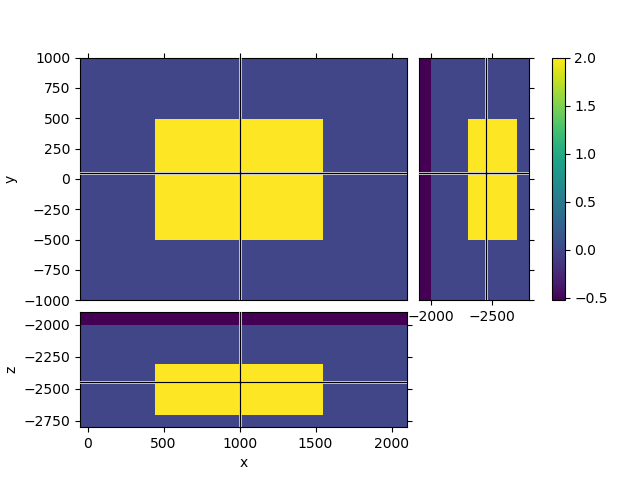
Put model on mesh

# Background model
mres_bg = np.ones(mesh.nC) * res_sea  # Upper halfspace; sea water
mres_bg[mesh.gridCC[:, 2] < seafloor] = res_bg  # Lower halfspace; background

# Target model
mres_tg = mres_bg.copy()  # Copy background model
target_inds = (  # Find target indices
    (mesh.gridCC[:, 0] >= tg_x[0])
    & (mesh.gridCC[:, 0] <= tg_x[1])
    & (mesh.gridCC[:, 1] >= tg_y[0])
    & (mesh.gridCC[:, 1] <= tg_y[1])
    & (mesh.gridCC[:, 2] >= tg_z[0])
    & (mesh.gridCC[:, 2] <= tg_z[1])
)
mres_tg[target_inds] = res_tg  # Target resistivity

# QC
mesh.plot_3d_slicer(
    np.log10(mres_tg),
    clim=[np.log10(res_sea), np.log10(res_tg)],
    xlim=[-src[0] - 100, rec[0] + 100],
    ylim=[-rec[0] / 2, rec[0] / 2],
    zlim=[tg_z[0] - 100, seafloor + 100],
)

Out:

/Users/josephcapriotti/opt/anaconda3/envs/py36/lib/python3.6/site-packages/discretize-0.4.11-py3.6-macosx-10.9-x86_64.egg/discretize/View.py:797: UserWarning: Matplotlib is currently using agg, which is a non-GUI backend, so cannot show the figure.
  plt.show()

(D) empymod

Compute the 1D background semi-analytically, using 5 points to approximate the 100-m long dipole.

inp = {
    "src": src.copy(),
    "rec": rec.copy(),
    "depth": seafloor,
    "res": [res_sea, res_bg],
    "freqtime": times,
    "signal": -1,  # Switch-off
    "srcpts": 5,  # 5 points for finite length approx
    "strength": 1,  # Account for source length
    "verb": 1,
}

epm_bg = empymod.bipole(**inp)

(E) SimPEG

Set-up SimPEG-specific parameters.

# Set up the receiver list
rec_list = [
    TDEM.Rx.PointElectricField(
        orientation="x", times=times, locs=np.array([[*rec[:3]],]),
    ),
]


# Set up the source list
src_list = [
    TDEM.Src.LineCurrent(rxList=rec_list, loc=np.array([[*src[::2]], [*src[1::2]]]),),
]


# Create `Survey`
survey = TDEM.Survey(src_list)


# Define the `Simulation`
prob = TDEM.Simulation3DElectricField(
    mesh,
    survey=survey,
    rhoMap=maps.IdentityMap(mesh),
    Solver=pymatsolver.Pardiso,
    timeSteps=time_steps,
)

Compute

spg_bg = prob.dpred(mres_bg)
spg_tg = prob.dpred(mres_tg)

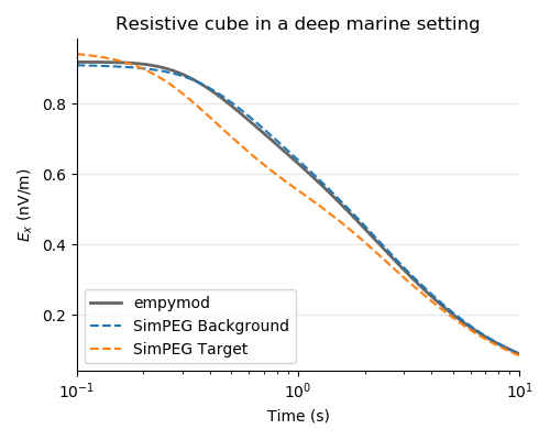
(F) Plots

plt.figure(figsize=(5, 4))
ax1 = plt.subplot(111)

plt.title("Resistive cube in a deep marine setting")

plt.plot(times, epm_bg * 1e9, ".4", lw=2, label="empymod")

plt.plot(times, spg_bg * 1e9, "C0--", label="SimPEG Background")
plt.plot(times, spg_tg * 1e9, "C1--", label="SimPEG Target")

plt.ylabel("$E_x$ (nV/m)")
plt.xscale("log")
plt.xlim([0.1, 10])
plt.legend(loc=3)
plt.grid(axis="y", c="0.9")

plt.xlabel("Time (s)")

# Switch off spines
ax1.spines["top"].set_visible(False)
ax1.spines["right"].set_visible(False)

plt.tight_layout()
plt.show()

Out:

/Users/josephcapriotti/codes/simpeg/examples/06-tdem/plot_fwd_tdem_3d_model.py:345: UserWarning: Matplotlib is currently using agg, which is a non-GUI backend, so cannot show the figure.
  plt.show()

empymod.Report([SimPEG, discretize, pymatsolver])

Tue May 26 19:12:42 2020 MDT
OS	Darwin	CPU(s)	8	Machine	x86_64
Architecture	64bit	Environment	Python
Python 3.6.10 |Anaconda, Inc.| (default, May 7 2020, 23:06:31) [GCC 4.2.1 Compatible Clang 4.0.1 (tags/RELEASE_401/final)]
SimPEG	0.14.0b2	discretize	0.4.11	pymatsolver	0.1.2
numpy	1.18.1	scipy	1.4.1	numba	0.49.1
empymod	2.0.0	IPython	7.13.0	matplotlib	3.1.3
Intel(R) Math Kernel Library Version 2019.0.4 Product Build 20190411 for Intel(R) 64 architecture applications