2.5D Forward Simulation of a DCIP Line

Here we use the module SimPEG.electromagnetics.static.resistivity to predict DC resistivity data and the module SimPEG.electromagnetics.static.induced_polarization to predict IP data for a dipole-dipole survey. In this tutorial, we focus on the following:

• How to define the survey

• How to define the problem

• How to predict DC resistivity data for a synthetic resistivity model

• How to predict IP data for a synthetic chargeability model

• How to include surface topography

• The units of the models and resulting data

This tutorial is split into two parts. First we create a resistivity model and predict DC resistivity data. Next we create a chargeability model and a background conductivity model to compute IP data.

Import modules

from discretize import TreeMesh
from discretize.utils import mkvc, refine_tree_xyz

from SimPEG.utils import model_builder, surface2ind_topo
from SimPEG import maps, data
from SimPEG.electromagnetics.static import resistivity as dc
from SimPEG.electromagnetics.static import induced_polarization as ip
from SimPEG.electromagnetics.static.utils import (
    generate_dcip_survey_line,
    plot_pseudoSection,
)

import os
import numpy as np
import matplotlib as mpl
import matplotlib.pyplot as plt

try:
    from pymatsolver import Pardiso as Solver
except ImportError:
    from SimPEG import SolverLU as Solver

save_file = False

# sphinx_gallery_thumbnail_number = 4

Defining Topography

Here we define surface topography as an (N, 3) numpy array. Topography could also be loaded from a file. In our case, our survey takes place in a valley that runs North-South.

x_topo, y_topo = np.meshgrid(
    np.linspace(-3000, 3000, 101), np.linspace(-3000, 3000, 101)
)
z_topo = (1 / np.pi) * 85 * (-np.pi / 2 + np.arctan((np.abs(x_topo) - 600.0) / 50.0))
x_topo, y_topo, z_topo = mkvc(x_topo), mkvc(y_topo), mkvc(z_topo)
xyz_topo = np.c_[x_topo, y_topo, z_topo]

Create Dipole-Dipole Survey

Here we define a single EW survey line that uses a dipole-dipole configuration. For the source, we must define the AB electrode locations. For the receivers we must define the MN electrode locations. Instead of creating the survey from scratch (see 1D example), we will use the generat_dcip_survey_line utility.

# Define survey line parameters
survey_type = "dipole-dipole"
data_type = "volt"
end_locations = np.r_[-400.0, 400]
station_separation = 50.0
dipole_separation = 25.0
n = 8

# Generate DC survey line
dc_survey = generate_dcip_survey_line(
    survey_type,
    data_type,
    end_locations,
    xyz_topo,
    station_separation,
    dipole_separation,
    n,
    dim_flag="2.5D",
    sources_only=False,
)

Create OcTree Mesh

Here, we create the OcTree mesh that will be used to predict both DC resistivity and IP data.

dh = 10.0  # base cell width
dom_width_x = 2400.0  # domain width x
dom_width_z = 1200.0  # domain width z
nbcx = 2 ** int(np.round(np.log(dom_width_x / dh) / np.log(2.0)))  # num. base cells x
nbcz = 2 ** int(np.round(np.log(dom_width_z / dh) / np.log(2.0)))  # num. base cells z

# Define the base mesh
hx = [(dh, nbcx)]
hz = [(dh, nbcz)]
mesh = TreeMesh([hx, hz], x0="CN")

# Mesh refinement based on topography
mesh = refine_tree_xyz(
    mesh, xyz_topo[:, [0, 2]], octree_levels=[1], method="surface", finalize=False
)

# Mesh refinement near transmitters and receivers. First we need to obtain the
# set of unique electrode locations.
electrode_locations = np.c_[
    dc_survey.locations_a,
    dc_survey.locations_b,
    dc_survey.locations_m,
    dc_survey.locations_n,
]

unique_locations = np.unique(
    np.reshape(electrode_locations, (4 * dc_survey.nD, 2)), axis=0
)

mesh = refine_tree_xyz(
    mesh, unique_locations, octree_levels=[2, 4], method="radial", finalize=False
)

# Refine core mesh region
xp, zp = np.meshgrid([-800.0, 800.0], [-800.0, 0.0])
xyz = np.c_[mkvc(xp), mkvc(zp)]
mesh = refine_tree_xyz(mesh, xyz, octree_levels=[0, 2, 2], method="box", finalize=False)

mesh.finalize()

Create Conductivity Model and Mapping for OcTree Mesh

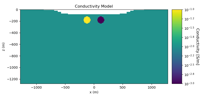
Here we define the conductivity model that will be used to predict DC resistivity data. The model consists of a conductive sphere and a resistive sphere within a moderately conductive background. Note that you can carry through this work flow with a resistivity model if desired.

# Define conductivity model in S/m (or resistivity model in Ohm m)
air_conductivity = 1e-8
background_conductivity = 1e-2
conductor_conductivity = 1e-1
resistor_conductivity = 1e-3

# Find active cells in forward modeling (cell below surface)
ind_active = surface2ind_topo(mesh, xyz_topo[:, [0, 2]])

# Define mapping from model to active cells
nC = int(ind_active.sum())
conductivity_map = maps.InjectActiveCells(mesh, ind_active, air_conductivity)

# Define model
conductivity_model = background_conductivity * np.ones(nC)

ind_conductor = model_builder.getIndicesSphere(np.r_[-120.0, -180.0], 60.0, mesh.gridCC)
ind_conductor = ind_conductor[ind_active]
conductivity_model[ind_conductor] = conductor_conductivity

ind_resistor = model_builder.getIndicesSphere(np.r_[120.0, -180.0], 60.0, mesh.gridCC)
ind_resistor = ind_resistor[ind_active]
conductivity_model[ind_resistor] = resistor_conductivity


# Plot Conductivity Model
fig = plt.figure(figsize=(8.5, 4))

plotting_map = maps.InjectActiveCells(mesh, ind_active, np.nan)
log_mod = np.log10(conductivity_model)

ax1 = fig.add_axes([0.1, 0.12, 0.73, 0.78])
mesh.plotImage(
    plotting_map * log_mod,
    ax=ax1,
    grid=False,
    clim=(np.log10(resistor_conductivity), np.log10(conductor_conductivity)),
    pcolorOpts={"cmap": "viridis"},
)
ax1.set_title("Conductivity Model")
ax1.set_xlabel("x (m)")
ax1.set_ylabel("z (m)")

ax2 = fig.add_axes([0.85, 0.12, 0.05, 0.78])
norm = mpl.colors.Normalize(
    vmin=np.log10(resistor_conductivity), vmax=np.log10(conductor_conductivity)
)
cbar = mpl.colorbar.ColorbarBase(
    ax2, norm=norm, cmap=mpl.cm.viridis, orientation="vertical", format="$10^{%.1f}$"
)
cbar.set_label("Conductivity [S/m]", rotation=270, labelpad=15, size=12)

Project Survey to Discretized Topography

It is important that electrodes are not model as being in the air. Even if the electrodes are properly located along surface topography, they may lie above the discretized topography. This step is carried out to ensure all electrodes like on the discretized surface.

dc_survey.drape_electrodes_on_topography(mesh, ind_active, option="top")

Predict DC Resistivity Data

Here we predict DC resistivity data. If the keyword argument sigmaMap is defined, the simulation will expect a conductivity model. If the keyword argument rhoMap is defined, the simulation will expect a resistivity model.

dc_simulation = dc.simulation_2d.Simulation2DNodal(
    mesh, survey=dc_survey, sigmaMap=conductivity_map, Solver=Solver
)

# Predict the data by running the simulation. The data are the raw voltage in
# units of volts.
dpred_dc = dc_simulation.dpred(conductivity_model)

# Define a data object (required for pseudo-section plot)
dc_data = data.Data(dc_survey, dobs=dpred_dc)

# Plot apparent conductivity pseudo-section
fig = plt.figure(figsize=(12, 5))

ax1 = fig.add_axes([0.05, 0.05, 0.8, 0.9])
plot_pseudoSection(
    dc_data,
    ax=ax1,
    survey_type="dipole-dipole",
    data_type="appConductivity",
    space_type="half-space",
    scale="log",
    pcolorOpts={"cmap": "viridis"},
)
ax1.set_title("Apparent Conductivity [S/m]")

plt.show()

Out:

/Users/josephcapriotti/codes/simpeg/tutorials/06-ip/plot_fwd_1_dcip2d.py:264: UserWarning: Matplotlib is currently using agg, which is a non-GUI backend, so cannot show the figure.
  plt.show()

Optional: Write out dpred

Write DC resistivity data, topography and true model

if save_file:

    dir_path = os.path.dirname(dc.__file__).split(os.path.sep)[:-4]
    dir_path.extend(["tutorials", "assets", "dcip2d"])
    dir_path = os.path.sep.join(dir_path) + os.path.sep

    # Add 5% Gaussian noise to each datum
    dc_noise = 0.05 * dpred_dc * np.random.rand(len(dpred_dc))

    # Write out data at their original electrode locations (not shifted)
    data_array = np.c_[electrode_locations, dpred_dc + dc_noise]

    fname = dir_path + "dc_data.obs"
    np.savetxt(fname, data_array, fmt="%.4e")

    fname = dir_path + "true_conductivity.txt"
    np.savetxt(fname, conductivity_map * conductivity_model, fmt="%.4e")

    fname = dir_path + "xyz_topo.txt"
    np.savetxt(fname, xyz_topo, fmt="%.4e")

Predict IP Resistivity Data

The geometry of the survey was defined earlier. Here, we use SimPEG functionality to make a copy for predicting IP data.

ip_survey = ip.from_dc_to_ip_survey(dc_survey, dim="2.5D")

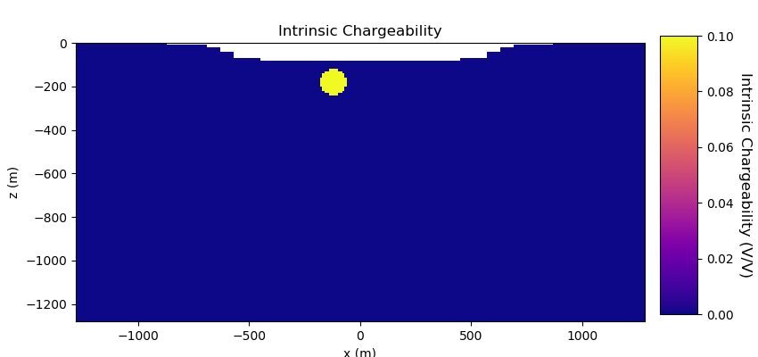
Create Chargeability Model and Mapping for OcTree Mesh

Here we define the chargeability model that will be used to predict IP data. Here we assume that the conductive sphere is also chargeable but the resistive sphere is not. Here, the chargeability is defined as mV/V.

# Define chargeability model as intrinsic chargeability (V/V).
air_chargeability = 0.0
background_chargeability = 0.0
sphere_chargeability = 1e-1

# Find active cells in forward modeling (cells below surface)
ind_active = surface2ind_topo(mesh, xyz_topo[:, [0, 2]])

# Define mapping from model to active cells
nC = int(ind_active.sum())
chargeability_map = maps.InjectActiveCells(mesh, ind_active, air_chargeability)

# Define chargeability model
chargeability_model = background_chargeability * np.ones(nC)

ind_chargeable = model_builder.getIndicesSphere(
    np.r_[-120.0, -180.0], 60.0, mesh.gridCC
)
ind_chargeable = ind_chargeable[ind_active]
chargeability_model[ind_chargeable] = sphere_chargeability

# Plot Chargeability Model
fig = plt.figure(figsize=(8.5, 4))

ax1 = fig.add_axes([0.1, 0.1, 0.75, 0.78])
mesh.plotImage(
    plotting_map * chargeability_model,
    ax=ax1,
    grid=False,
    pcolorOpts={"cmap": "plasma"},
)
ax1.set_title("Intrinsic Chargeability")
ax1.set_xlabel("x (m)")
ax1.set_ylabel("z (m)")

ax2 = fig.add_axes([0.87, 0.12, 0.05, 0.78])
norm = mpl.colors.Normalize(vmin=0, vmax=sphere_chargeability)
cbar = mpl.colorbar.ColorbarBase(
    ax2, norm=norm, orientation="vertical", cmap=mpl.cm.plasma
)
cbar.set_label("Intrinsic Chargeability (V/V)", rotation=270, labelpad=15, size=12)

Predict IP Data

Here we use a chargeability model and a background conductivity/resistivity model to predict IP data.

# We use the keyword argument *sigma* to define the background conductivity on
# the mesh. We could use the keyword argument *rho* to accomplish the same thing
# using a background resistivity model.
simulation_ip = ip.simulation_2d.Simulation2DNodal(
    mesh,
    survey=ip_survey,
    etaMap=chargeability_map,
    sigma=conductivity_map * conductivity_model,
    Solver=Solver,
)

# Run forward simulation and predicted IP data. The data are the voltage (V)
dpred_ip = simulation_ip.dpred(chargeability_model)

# Define a data object. Required for pseudo-section plot
ip_data = data.Data(ip_survey, dobs=dpred_ip)

# Plot apparent chargeability. To accomplish this, we must normalize the IP
# voltage by the DC voltage. This is then multiplied by 1000 so that our
# apparent chargeability is in units mV/V.
fig = plt.figure(figsize=(12, 9))

# Plot apparent conductivity
ax1 = fig.add_axes([0.05, 0.55, 0.8, 0.42])
plot_pseudoSection(
    dc_data,
    ax=ax1,
    survey_type="dipole-dipole",
    data_type="appConductivity",
    space_type="half-space",
    scale="log",
    pcolorOpts={"cmap": "viridis"},
)
ax1.set_title("Apparent Conductivity [S/m]")

# Convert from voltage measurement to apparent chargeability by normalizing by
# the DC voltage
apparent_chargeability = dpred_ip / dpred_dc

ax2 = fig.add_axes([0.05, 0.05, 0.8, 0.42])
plot_pseudoSection(
    ip_data,
    dobs=apparent_chargeability,
    ax=ax2,
    survey_type="dipole-dipole",
    data_type="appChargeability",
    space_type="half-space",
    scale="linear",
    pcolorOpts={"cmap": "plasma"},
)
ax2.set_title("Apparent Chargeability (V/V)")

plt.show()

Out:

/Users/josephcapriotti/codes/simpeg/tutorials/06-ip/plot_fwd_1_dcip2d.py:416: UserWarning: Matplotlib is currently using agg, which is a non-GUI backend, so cannot show the figure.
  plt.show()

Write out dpred

Write data and true model

if save_file:

    # Add 1% Gaussian noise based on the DC data (not the IP data)
    ip_noise = 0.01 * np.abs(dpred_dc) * np.random.rand(len(dpred_ip))

    data_array = np.c_[electrode_locations, dpred_ip + ip_noise]

    fname = dir_path + "ip_data.obs"
    np.savetxt(fname, data_array, fmt="%.4e")

    fname = dir_path + "true_chargeability.txt"
    np.savetxt(fname, chargeability_map * chargeability_model, fmt="%.4e")