Forward Simulation on a Tree Mesh

Here we use the module SimPEG.electromagnetics.frequency_domain to simulate the FDEM response for an airborne survey using an OcTree mesh and a conductivity/resistivity model. To limit computational demant, we simulate airborne data at a single frequency for a vertical coplanar survey geometry. This tutorial can be easily adapted to simulate data at many frequencies. For this tutorial, we focus on the following:

• How to define the transmitters and receivers

• How to define the survey

• How to define the topography

• How to solve the FDEM problem on OcTree meshes

• The units of the conductivity/resistivity model and resulting data

Please note that we have used a coarse mesh to shorten the time of the simulation. Proper discretization is required to simulate the fields at each frequency with sufficient accuracy.

Import modules

from discretize import TreeMesh
from discretize.utils import mkvc, refine_tree_xyz

from SimPEG.utils import plot2Ddata, surface2ind_topo
from SimPEG import maps
import SimPEG.electromagnetics.frequency_domain as fdem

import os
import numpy as np
import matplotlib as mpl
import matplotlib.pyplot as plt

try:
    from pymatsolver import Pardiso as Solver
except ImportError:
    from SimPEG import SolverLU as Solver

save_file = False

# sphinx_gallery_thumbnail_number = 2

Defining Topography

Here we define surface topography as an (N, 3) numpy array. Topography could also be loaded from a file. Here we define flat topography, however more complex topographies can be considered.

xx, yy = np.meshgrid(np.linspace(-3000, 3000, 101), np.linspace(-3000, 3000, 101))
zz = np.zeros(np.shape(xx))
topo_xyz = np.c_[mkvc(xx), mkvc(yy), mkvc(zz)]

Create Airborne Survey

For this example, the survey consists of a uniform grid of airborne measurements. To save time, we will only compute the response for a single frequency.

# Frequencies being predicted
frequencies = [100, 500, 2500]

# Defining transmitter locations
N = 9
xtx, ytx, ztx = np.meshgrid(np.linspace(-200, 200, N), np.linspace(-200, 200, N), [40])
source_locations = np.c_[mkvc(xtx), mkvc(ytx), mkvc(ztx)]
ntx = np.size(xtx)

# Define receiver locations
xrx, yrx, zrx = np.meshgrid(np.linspace(-200, 200, N), np.linspace(-200, 200, N), [20])
receiver_locations = np.c_[mkvc(xrx), mkvc(yrx), mkvc(zrx)]

source_list = []  # Create empty list to store sources

# Each unique location and frequency defines a new transmitter
for ii in range(len(frequencies)):
    for jj in range(ntx):

        # Define receivers of different type at each location
        bzr_receiver = fdem.receivers.PointMagneticFluxDensitySecondary(
            receiver_locations[jj, :], "z", "real"
        )
        bzi_receiver = fdem.receivers.PointMagneticFluxDensitySecondary(
            receiver_locations[jj, :], "z", "imag"
        )
        receivers_list = [bzr_receiver, bzi_receiver]

        # Must define the transmitter properties and associated receivers
        source_list.append(
            fdem.sources.MagDipole(
                receivers_list,
                frequencies[ii],
                source_locations[jj],
                orientation="z",
                moment=100,
            )
        )

survey = fdem.Survey(source_list)

Create OcTree Mesh

Here we define the OcTree mesh that is used for this example. We chose to design a coarser mesh to decrease the run time. When designing a mesh to solve practical frequency domain problems:

• Your smallest cell size should be 10%-20% the size of your smallest skin depth

• The thickness of your padding needs to be 2-3 times biggest than your largest skin depth

• The skin depth is ~500*np.sqrt(rho/f)

dh = 25.0  # base cell width
dom_width = 3000.0  # domain width
nbc = 2 ** int(np.round(np.log(dom_width / dh) / np.log(2.0)))  # num. base cells

# Define the base mesh
h = [(dh, nbc)]
mesh = TreeMesh([h, h, h], x0="CCC")

# Mesh refinement based on topography
mesh = refine_tree_xyz(
    mesh, topo_xyz, octree_levels=[0, 0, 0, 1], method="surface", finalize=False
)

# Mesh refinement near transmitters and receivers
mesh = refine_tree_xyz(
    mesh, receiver_locations, octree_levels=[2, 4], method="radial", finalize=False
)

# Refine core mesh region
xp, yp, zp = np.meshgrid([-250.0, 250.0], [-250.0, 250.0], [-300.0, 0.0])
xyz = np.c_[mkvc(xp), mkvc(yp), mkvc(zp)]
mesh = refine_tree_xyz(mesh, xyz, octree_levels=[0, 2, 4], method="box", finalize=False)

mesh.finalize()

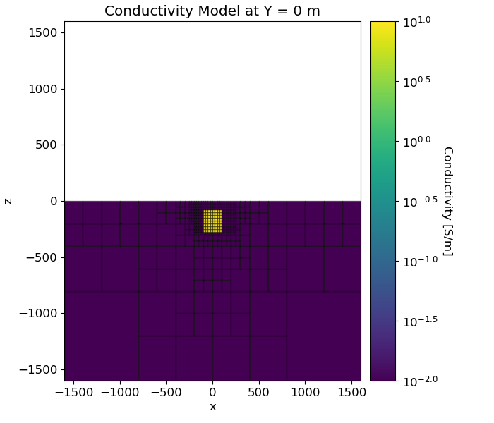
Defining the Conductivity/Resistivity Model and Mapping

Here, we create the model that will be used to predict frequency domain data and the mapping from the model to the mesh. Here, the model consists of a conductive block within a more resistive background.

# Conductivity in S/m (or resistivity in Ohm m)
air_conductivity = 1e-8
background_conductivity = 1e-2
block_conductivity = 1e1

# Find cells that are active in the forward modeling (cells below surface)
ind_active = surface2ind_topo(mesh, topo_xyz)

# Define mapping from model to active cells
model_map = maps.InjectActiveCells(mesh, ind_active, air_conductivity)

# Define model. Models in SimPEG are vector arrays
model = background_conductivity * np.ones(ind_active.sum())
ind_block = (
    (mesh.gridCC[ind_active, 0] < 100.0)
    & (mesh.gridCC[ind_active, 0] > -100.0)
    & (mesh.gridCC[ind_active, 1] < 100.0)
    & (mesh.gridCC[ind_active, 1] > -100.0)
    & (mesh.gridCC[ind_active, 2] > -275.0)
    & (mesh.gridCC[ind_active, 2] < -75.0)
)
model[ind_block] = block_conductivity

# Plot Resistivity Model
mpl.rcParams.update({"font.size": 12})
fig = plt.figure(figsize=(7, 6))

plotting_map = maps.InjectActiveCells(mesh, ind_active, np.nan)
log_model = np.log10(model)

ax1 = fig.add_axes([0.13, 0.1, 0.6, 0.85])
mesh.plotSlice(
    plotting_map * log_model,
    normal="Y",
    ax=ax1,
    ind=int(mesh.hx.size / 2),
    grid=True,
    clim=(np.log10(background_conductivity), np.log10(block_conductivity)),
)
ax1.set_title("Conductivity Model at Y = 0 m")

ax2 = fig.add_axes([0.75, 0.1, 0.05, 0.85])
norm = mpl.colors.Normalize(
    vmin=np.log10(background_conductivity), vmax=np.log10(block_conductivity)
)
cbar = mpl.colorbar.ColorbarBase(
    ax2, norm=norm, orientation="vertical", format="$10^{%.1f}$"
)
cbar.set_label("Conductivity [S/m]", rotation=270, labelpad=15, size=12)

Simulation: Predicting FDEM Data

Here we define the formulation for solving Maxwell’s equations. Since we are measuring the magnetic flux density and working with a conductivity model, the EB formulation is the most natural. We must also remember to define the mapping for the conductivity model. If you defined a resistivity model, use the kwarg rhoMap instead of sigmaMap

simulation = fdem.simulation.Simulation3DMagneticFluxDensity(
    mesh, survey=survey, sigmaMap=model_map, Solver=Solver
)

Predict and Plot Data

Here we show how the simulation is used to predict data.

# Compute predicted data for a your model.
dpred = simulation.dpred(model)

# Data are organized by frequency, transmitter location, then by receiver. We nFreq transmitters
# and each transmitter had 2 receivers (real and imaginary component). So
# first we will pick out the real and imaginary data
bz_real = dpred[0 : len(dpred) : 2]
bz_imag = dpred[1 : len(dpred) : 2]

# Then we will will reshape the data for plotting.
bz_real_plotting = np.reshape(bz_real, (len(frequencies), ntx))
bz_imag_plotting = np.reshape(bz_imag, (len(frequencies), ntx))

fig = plt.figure(figsize=(10, 4))

# Real Component
frequencies_index = 0
v_max = np.max(np.abs(bz_real_plotting[frequencies_index, :]))
ax1 = fig.add_axes([0.05, 0.05, 0.35, 0.9])
plot2Ddata(
    receiver_locations[:, 0:2],
    bz_real_plotting[frequencies_index, :],
    ax=ax1,
    ncontour=30,
    clim=(-v_max, v_max),
    contourOpts={"cmap": "bwr"},
)
ax1.set_title("Re[$B_z$] at 100 Hz")

ax2 = fig.add_axes([0.41, 0.05, 0.02, 0.9])
norm = mpl.colors.Normalize(vmin=-v_max, vmax=v_max)
cbar = mpl.colorbar.ColorbarBase(
    ax2, norm=norm, orientation="vertical", cmap=mpl.cm.bwr
)
cbar.set_label("$T$", rotation=270, labelpad=15, size=12)

# Imaginary Component
v_max = np.max(np.abs(bz_imag_plotting[frequencies_index, :]))
ax1 = fig.add_axes([0.55, 0.05, 0.35, 0.9])
plot2Ddata(
    receiver_locations[:, 0:2],
    bz_imag_plotting[frequencies_index, :],
    ax=ax1,
    ncontour=30,
    clim=(-v_max, v_max),
    contourOpts={"cmap": "bwr"},
)
ax1.set_title("Im[$B_z$] at 100 Hz")

ax2 = fig.add_axes([0.91, 0.05, 0.02, 0.9])
norm = mpl.colors.Normalize(vmin=-v_max, vmax=v_max)
cbar = mpl.colorbar.ColorbarBase(
    ax2, norm=norm, orientation="vertical", cmap=mpl.cm.bwr
)
cbar.set_label("$T$", rotation=270, labelpad=15, size=12)

plt.show()

Out:

/Users/josephcapriotti/codes/simpeg/tutorials/07-fdem/plot_fwd_3_fem_3d.py:294: UserWarning: Matplotlib is currently using agg, which is a non-GUI backend, so cannot show the figure.
  plt.show()

Optional: Export Data

Write the true model, data and topography

if save_file:

    dir_path = os.path.dirname(fdem.__file__).split(os.path.sep)[:-3]
    dir_path.extend(["tutorials", "assets", "fdem"])
    dir_path = os.path.sep.join(dir_path) + os.path.sep

    # Write topography
    fname = dir_path + "fdem_topo.txt"
    np.savetxt(fname, np.c_[topo_xyz], fmt="%.4e")

    # Write data with 2% noise added
    fname = dir_path + "fdem_data.obs"
    bz_real = bz_real + 1e-14 * np.random.rand(len(bz_real))
    bz_imag = bz_imag + 1e-14 * np.random.rand(len(bz_imag))
    f_vec = np.kron(frequencies, np.ones(ntx))
    receiver_locations = np.kron(np.ones((len(frequencies), 1)), receiver_locations)

    np.savetxt(fname, np.c_[f_vec, receiver_locations, bz_real, bz_imag], fmt="%.4e")

    # Plot true model
    output_model = plotting_map * model
    output_model[np.isnan(output_model)] = 1e-8

    fname = dir_path + "true_model.txt"
    np.savetxt(fname, output_model, fmt="%.4e")