Forward Simulation for Transient Response on a Cylindrical Mesh

Here we use the module SimPEG.electromagnetics.time_domain to simulate the transient response for an airborne survey using a cylindrical mesh and a conductivity model. We simulate a single line of airborne data at many time channels for a vertical coplanar survey geometry. For this tutorial, we focus on the following:

• How to define the transmitters and receivers

• How to define the transmitter waveform for a step-off

• How to define the time-stepping

• How to define the survey

• How to solve TDEM problems on a cylindrical mesh

• The units of the conductivity/resistivity model and resulting data

Please note that we have used a coarse mesh larger time-stepping to shorten the time of the simulation. Proper discretization in space and time is required to simulate the fields at each time channel with sufficient accuracy.

Import Modules

from discretize import CylMesh
from discretize.utils import mkvc

from SimPEG import maps
import SimPEG.electromagnetics.time_domain as tdem

import numpy as np
import matplotlib as mpl
import matplotlib.pyplot as plt

try:
    from pymatsolver import Pardiso as Solver
except ImportError:
    from SimPEG import SolverLU as Solver

write_file = False

# sphinx_gallery_thumbnail_number = 2

Defining the Waveform

Under SimPEG.electromagnetic.time_domain.sources there are a multitude of waveforms that can be defined (VTEM, Ramp-off etc…). Here we simulate the response due to a step off waveform where the off-time begins at t=0. Other waveforms are discuss in the OcTree simulation example.

waveform = tdem.sources.StepOffWaveform(offTime=0.0)

Create Airborne Survey

Here we define the survey used in our simulation. For time domain simulations, we must define the geometry of the source and its waveform. For the receivers, we define their geometry, the type of field they measure and the time channels at which they measure the field. For this example, the survey consists of a uniform grid of airborne measurements.

# Observation times for response (time channels)
time_channels = np.logspace(-4, -2, 11)

# Defining transmitter locations
xtx, ytx, ztx = np.meshgrid(np.linspace(0, 200, 41), [0], [55])
source_locations = np.c_[mkvc(xtx), mkvc(ytx), mkvc(ztx)]
ntx = np.size(xtx)

# Define receiver locations
xrx, yrx, zrx = np.meshgrid(np.linspace(0, 200, 41), [0], [50])
receiver_locations = np.c_[mkvc(xrx), mkvc(yrx), mkvc(zrx)]

source_list = []  # Create empty list to store sources

# Each unique location defines a new transmitter
for ii in range(ntx):

    # Define receivers at each location.
    dbzdt_receiver = tdem.receivers.PointMagneticFluxTimeDerivative(
        receiver_locations[ii, :], time_channels, "z"
    )
    receivers_list = [
        dbzdt_receiver
    ]  # Make a list containing all receivers even if just one

    # Must define the transmitter properties and associated receivers
    source_list.append(
        tdem.sources.MagDipole(
            receivers_list,
            location=source_locations[ii],
            waveform=waveform,
            moment=1.0,
            orientation="z",
        )
    )

survey = tdem.Survey(source_list)

Create Cylindrical Mesh

Here we create the cylindrical mesh that will be used for this tutorial example. We chose to design a coarser mesh to decrease the run time. When designing a mesh to solve practical time domain problems:

• Your smallest cell size should be 10%-20% the size of your smallest diffusion distance

• The thickness of your padding needs to be 2-3 times biggest than your largest diffusion distance

• The diffusion distance is ~1260*np.sqrt(rho*t)

hr = [(10.0, 50), (10.0, 10, 1.5)]
hz = [(10.0, 10, -1.5), (10.0, 100), (10.0, 10, 1.5)]

mesh = CylMesh([hr, 1, hz], x0="00C")

Create Conductivity/Resistivity Model and Mapping

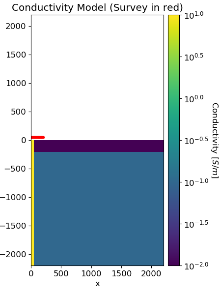
Here, we create the model that will be used to predict time domain data and the mapping from the model to the mesh. The model consists of a long vertical conductive pipe and a resistive surface layer. For this example, we will have only flat topography.

# Conductivity in S/m (or resistivity in Ohm m)
air_conductivity = 1e-8
background_conductivity = 1e-1
layer_conductivity = 1e-2
pipe_conductivity = 1e1

# Find cells that are active in the forward modeling (cells below surface)
ind_active = mesh.gridCC[:, 2] < 0

# Define mapping from model to active cells
model_map = maps.InjectActiveCells(mesh, ind_active, air_conductivity)

# Define the model
model = background_conductivity * np.ones(ind_active.sum())
ind_layer = (mesh.gridCC[ind_active, 2] > -200.0) & (mesh.gridCC[ind_active, 2] < -0)
model[ind_layer] = layer_conductivity
ind_pipe = (
    (mesh.gridCC[ind_active, 0] < 50.0)
    & (mesh.gridCC[ind_active, 2] > -10000.0)
    & (mesh.gridCC[ind_active, 2] < 0.0)
)
model[ind_pipe] = pipe_conductivity


# Plot Resistivity Model
mpl.rcParams.update({"font.size": 12})
fig = plt.figure(figsize=(4.5, 6))

plotting_map = maps.InjectActiveCells(mesh, ind_active, np.nan)
log_model = np.log10(model)  # So scaling is log-scale

ax1 = fig.add_axes([0.14, 0.1, 0.6, 0.85])
mesh.plotImage(
    plotting_map * log_model,
    ax=ax1,
    grid=False,
    clim=(np.log10(layer_conductivity), np.log10(pipe_conductivity)),
)
ax1.set_title("Conductivity Model (Survey in red)")

ax1.plot(receiver_locations[:, 0], receiver_locations[:, 2], "r.")

ax2 = fig.add_axes([0.76, 0.1, 0.05, 0.85])
norm = mpl.colors.Normalize(
    vmin=np.log10(layer_conductivity), vmax=np.log10(pipe_conductivity)
)
cbar = mpl.colorbar.ColorbarBase(
    ax2, norm=norm, orientation="vertical", format="$10^{%.1f}$"
)
cbar.set_label("Conductivity [$S/m$]", rotation=270, labelpad=15, size=12)

Define the Time-Stepping

Stuff about time-stepping and some rule of thumb for step-off waveform

time_steps = [(5e-06, 20), (0.0001, 20), (0.001, 21)]

Define the Simulation

Here we define the formulation for solving Maxwell’s equations. Since we are measuring the time-derivative of the magnetic flux density and working with a conductivity model, the EB formulation is the most natural. We must also remember to define the mapping for the conductivity model. Use rhoMap instead of sigmaMap if you defined a resistivity model.

simulation = tdem.simulation.Simulation3DMagneticFluxDensity(
    mesh, survey=survey, sigmaMap=model_map, Solver=Solver
)

# Set the time-stepping for the simulation
simulation.time_steps = time_steps

Predict Data and Plot

# Data are organized by transmitter, then by
# receiver then by observation time. dBdt data are in T/s.
dpred = simulation.dpred(model)

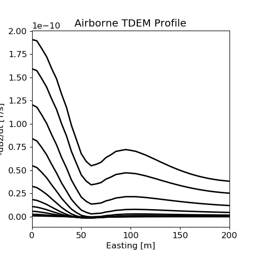
# Plot the response
dpred = np.reshape(dpred, (ntx, len(time_channels)))

# TDEM Profile
fig = plt.figure(figsize=(5, 5))
ax1 = fig.add_subplot(111)
for ii in range(0, len(time_channels)):
    ax1.plot(
        receiver_locations[:, 0], -dpred[:, ii], "k", lw=2
    )  # -ve sign to plot -dBz/dt
ax1.set_xlim((0, np.max(xtx)))
ax1.set_xlabel("Easting [m]")
ax1.set_ylabel("-dBz/dt [T/s]")
ax1.set_title("Airborne TDEM Profile")

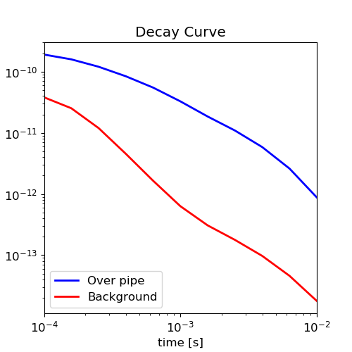
# Response over pipe for all time channels
fig = plt.figure(figsize=(5, 5))
ax1 = fig.add_subplot(111)
ax1.loglog(time_channels, -dpred[0, :], "b", lw=2)
ax1.loglog(time_channels, -dpred[-1, :], "r", lw=2)
ax1.set_xlim((np.min(time_channels), np.max(time_channels)))
ax1.set_xlabel("time [s]")
ax1.set_ylabel("-dBz/dt [T/s]")
ax1.set_title("Decay Curve")
ax1.legend(["Over pipe", "Background"], loc="lower left")

• 
• 

Out:

<matplotlib.legend.Legend object at 0x182edc25c0>