Forward Simulation for Straight Ray Tomography in 2D

Here we module SimPEG.seismic.straight_ray_tomography to predict arrival time data for a synthetic velocity/slowness model. In this tutorial, we focus on the following:

• How to define the survey

• How to define the forward simulation

• How to predict arrival time data

Import Modules

import os
import numpy as np
import matplotlib as mpl
import matplotlib.pyplot as plt

from discretize import TensorMesh

from SimPEG import maps
from SimPEG.seismic import straight_ray_tomography as tomo
from SimPEG.utils import model_builder

save_file = False

Defining the Survey

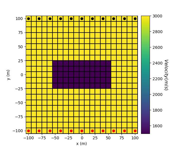
Here, we define survey that will be used for the forward simulation. The survey consists of a horizontal line of point receivers at Y = 100 m and a horizontal line of point sources at Y = -100 m. The shot by each source is measured by all receivers.

# Define the locations for the sources and receivers.
x = np.linspace(-100, 100, 11)
y_receivers = 100 * np.ones(len(x))
y_sources = -100 * np.ones(len(x))

receiver_locations = np.c_[x, y_receivers]
source_locations = np.c_[x, y_sources]

# Define the list of receivers used by each source
receiver_list = [tomo.Rx(receiver_locations)]

# Define an empty list to store sources objects. Define each source and
# provide its corresponding receivers list
source_list = []
for ii in range(0, len(y_sources)):
    source_list.append(
        tomo.Src(location=source_locations[ii, :], receiver_list=receiver_list)
    )

# Define they tomography survey
survey = tomo.Survey(source_list)

Defining a Tensor Mesh

Here, we create the tensor mesh that will be used to predict arrival time data.

dh = 10.0  # cell width
N = 21  # number of cells in X and Y direction
hx = [(dh, N)]
hy = [(dh, N)]
mesh = TensorMesh([hx, hy], "CC")

Model and Mapping on Tensor Mesh

Here, we create the velocity model that will be used to predict the data. Since the physical parameter for straight ray tomography is slowness, we must define a mapping which converts velocity values to slowness values. The model consists of a lower velocity block within a higher velocity background.

# Define velocity of each unit in m/s
background_velocity = 3000.0
block_velocity = 1500.0

# Define the model. Models in SimPEG are vector arrays.
model = background_velocity * np.ones(mesh.nC)

ind_block = model_builder.getIndicesBlock(np.r_[-50, 20], np.r_[50, -20], mesh.gridCC)
model[ind_block] = block_velocity

# Define a mapping from the model (velocity) to the slowness. If your model
# consists of slowness values, you can use *maps.IdentityMap*.
model_mapping = maps.ReciprocalMap()

# Plot Velocity Model
fig = plt.figure(figsize=(6, 5.5))

ax1 = fig.add_axes([0.15, 0.15, 0.65, 0.75])
mesh.plotImage(model, ax=ax1, grid=True, pcolorOpts={"cmap": "viridis"})
ax1.set_xlabel("x (m)")
ax1.set_ylabel("y (m)")
ax1.plot(x, y_sources, "ro")  # source locations
ax1.plot(x, y_receivers, "ko")  # receiver locations

ax2 = fig.add_axes([0.82, 0.15, 0.05, 0.75])
norm = mpl.colors.Normalize(vmin=np.min(model), vmax=np.max(model))
cbar = mpl.colorbar.ColorbarBase(
    ax2, norm=norm, orientation="vertical", cmap=mpl.cm.viridis
)
cbar.set_label("$Velocity (m/s)$", rotation=270, labelpad=15, size=12)

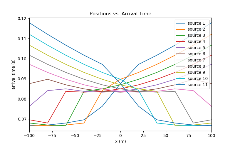
Simulation: Arrival Time

Here we demonstrate how to predict arrival time data for the 2D straight ray tomography problem using the 2D Integral formulation.

# Define the forward simulation. To do this we need the mesh, the survey and
# the mapping from the model to the slowness values on the mesh.
simulation = tomo.Simulation(mesh, survey=survey, slownessMap=model_mapping)

# Compute predicted data for some model
dpred = simulation.dpred(model)

Plotting

n_source = len(source_list)
n_receiver = len(x)
dpred_plotting = dpred.reshape(n_receiver, n_source)

fig = plt.figure(figsize=(8, 5))
ax = fig.add_subplot(111)
obs_string = []

for ii in range(0, n_source):
    ax.plot(x, dpred_plotting[:, ii])
    obs_string.append("source {}".format(ii + 1))

ax.set_xlim(np.min(x), np.max(x))
ax.set_xlabel("x (m)")
ax.set_ylabel("arrival time (s)")
ax.set_title("Positions vs. Arrival Time")
ax.legend(obs_string, loc="upper right")

Out:

<matplotlib.legend.Legend object at 0xd24454c18>

Optional: Exporting Results

Write the data and true model

if save_file:

    dir_path = os.path.dirname(tomo.__file__).split(os.path.sep)[:-3]
    dir_path.extend(["tutorials", "seismic", "assets"])
    dir_path = os.path.sep.join(dir_path) + os.path.sep

    noise = 0.05 * dpred * np.random.rand(len(dpred))

    data_array = np.c_[
        np.kron(x, np.ones(n_receiver)),
        np.kron(y_sources, np.ones(n_receiver)),
        np.kron(np.ones(n_source), x),
        np.kron(np.ones(n_source), y_receivers),
        dpred + noise,
    ]

    fname = dir_path + "tomography2D_data.obs"
    np.savetxt(fname, data_array, fmt="%.4e")

    output_model = model
    fname = dir_path + "true_model_2D.txt"
    np.savetxt(fname, output_model, fmt="%.4e")