Utils

Matrix Utilities

SimPEG.utils.mat_utils.diagEst(matFun, n, k=None, approach='Probing')

Estimate the diagonal of a matrix, A. Note that the matrix may be a function which returns A times a vector.

Three different approaches have been implemented:

1. Probing: cyclic permutations of vectors with 1’s and 0’s (default)

2. Ones: random +/- 1 entries

3. Random: random vectors

Parameters

• matFun (callable) – takes a (numpy.ndarray) and multiplies it by a matrix to estimate the diagonal

• n (int) – size of the vector that should be used to compute matFun(v)

• k (int) – number of vectors to be used to estimate the diagonal

• approach (str) – approach to be used for getting vectors

Return type

numpy.ndarray

Returns

est_diag(A)

Based on Saad http://www-users.cs.umn.edu/~saad/PDF/umsi-2005-082.pdf, and https://www.cita.utoronto.ca/~niels/diagonal.pdf

SimPEG.utils.mat_utils.uniqueRows(M)

SimPEG.utils.mat_utils.cartesian2spherical(m)

Convert from cartesian to spherical

SimPEG.utils.mat_utils.spherical2cartesian(m)

Convert from spherical to cartesian

SimPEG.utils.mat_utils.dip_azimuth2cartesian(dip, azm_N)

Function converting degree angles for dip and azimuth from north to a 3-components in cartesian coordinates.

INPUT dip : Value or vector of dip from horizontal in DEGREE azm_N : Value or vector of azimuth from north in DEGREE

OUTPUT M : [n-by-3] Array of xyz components of a unit vector in cartesian

Created on Dec, 20th 2015

@author: dominiquef

SimPEG.utils.mat_utils.coterminal(theta)

Compute coterminal angle so that [-pi < theta < pi]

Solver Utilities

SimPEG.utils.solver_utils.SolverWrapD(fun, factorize=True, checkAccuracy=True, accuracyTol=1e-06, name=None)

Wraps a direct Solver.

import scipy.sparse as sp
Solver   = solver_utils.SolverWrapD(sp.linalg.spsolve, factorize=False)
SolverLU = solver_utils.SolverWrapD(sp.linalg.splu, factorize=True)

SimPEG.utils.solver_utils.SolverWrapI(fun, checkAccuracy=True, accuracyTol=1e-05, name=None)

Wraps an iterative Solver.

import scipy.sparse as sp
SolverCG = solver_utils.SolverWrapI(sp.linalg.cg)

class SimPEG.utils.solver_utils.Solver(A, **kwargs)

clean()

class SimPEG.utils.solver_utils.SolverLU(A, **kwargs)

clean()

class SimPEG.utils.solver_utils.SolverCG(A, **kwargs)

clean()

class SimPEG.utils.solver_utils.SolverBiCG(A, **kwargs)

clean()

class SimPEG.utils.solver_utils.SolverDiag(A, **kwargs)

docstring for SolverDiag

clean()

Curv Utilities

Mesh Utilities

Model Builder Utilities

SimPEG.utils.model_builder.addBlock(gridCC, modelCC, p0, p1, blockProp)

Add a block to an exsisting cell centered model, modelCC

Parameters

• gridCC (numpy.ndarray) – mesh.gridCC is the cell centered grid

• modelCC (numpy.ndarray) – cell centered model

• p0 (numpy.ndarray) – bottom, southwest corner of block

• p1 (numpy.ndarray) – top, northeast corner of block

BlockProp float blockProp

property to assign to the model

Return numpy.ndarray, modelBlock

model with block

SimPEG.utils.model_builder.getIndicesBlock(p0, p1, ccMesh)

Creates a vector containing the block indices in the cell centers mesh. Returns a tuple

The block is defined by the points

p0, describe the position of the left upper front corner, and

p1, describe the position of the right bottom back corner.

ccMesh represents the cell-centered mesh

The points p0 and p1 must live in the the same dimensional space as the mesh.

SimPEG.utils.model_builder.defineBlock(ccMesh, p0, p1, vals=None)

Build a block with the conductivity specified by condVal. Returns an array. vals[0] conductivity of the block vals[1] conductivity of the ground

SimPEG.utils.model_builder.defineElipse(ccMesh, center=None, anisotropy=None, slope=10.0, theta=0.0)

SimPEG.utils.model_builder.getIndicesSphere(center, radius, ccMesh)

Creates a vector containing the sphere indices in the cell centers mesh. Returns a tuple

The sphere is defined by the points

p0, describe the position of the center of the cell

r, describe the radius of the sphere.

ccMesh represents the cell-centered mesh

The points p0 must live in the the same dimensional space as the mesh.

SimPEG.utils.model_builder.defineTwoLayers(ccMesh, depth, vals=None)

Define a two layered model. Depth of the first layer must be specified. CondVals vector with the conductivity values of the layers. Eg:

Convention to number the layers:

<----------------------------|------------------------------------>
0                          depth                                 zf
     1st layer                       2nd layer

SimPEG.utils.model_builder.scalarConductivity(ccMesh, pFunction)

Define the distribution conductivity in the mesh according to the analytical expression given in pFunction

SimPEG.utils.model_builder.layeredModel(ccMesh, layerTops, layerValues)

Define a layered model from layerTops (z-positive up)

Parameters

• ccMesh (numpy.ndarray) – cell-centered mesh

• layerTops (numpy.ndarray) – z-locations of the tops of each layer

• layerValue (numpy.ndarray) – values of the property to assign for each layer (starting at the top)

Return type

numpy.ndarray

Returns

M, layered model on the mesh

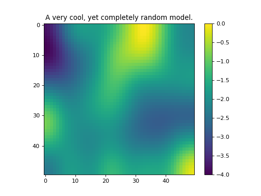
SimPEG.utils.model_builder.randomModel(shape, seed=None, anisotropy=None, its=100, bounds=None)

Create a random model by convolving a kernel with a uniformly distributed model.

Parameters

• shape (tuple) – shape of the model.

• seed (int) – pick which model to produce, prints the seed if you don’t choose.

• anisotropy (numpy.ndarray) – this is the (3 x n) blurring kernel that is used.

• its (int) – number of smoothing iterations

• bounds (list) – bounds on the model, len(list) == 2

Return type

numpy.ndarray

Returns

M, the model

(Source code, png, hires.png, pdf)

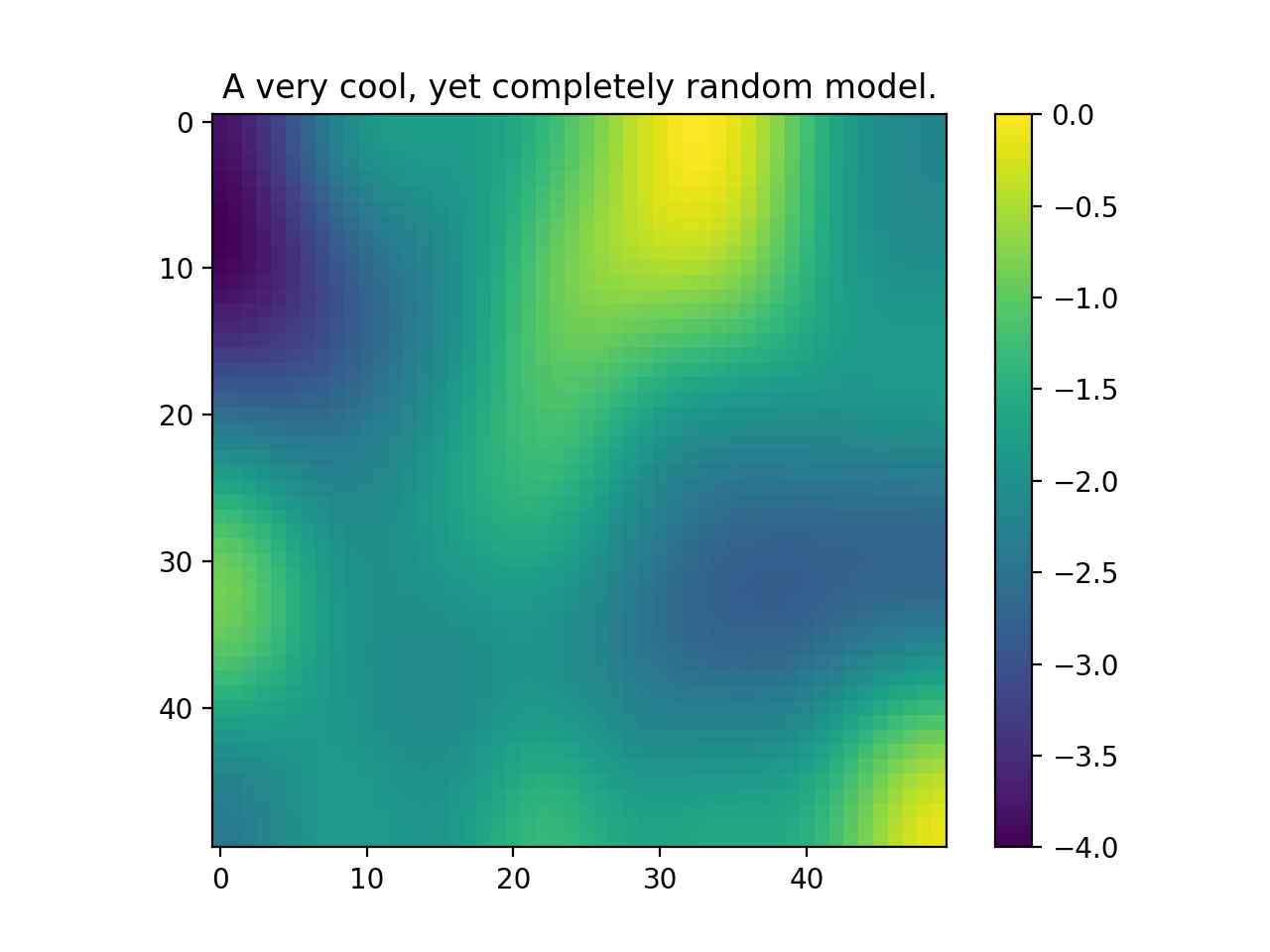
SimPEG.utils.model_builder.PolygonInd(mesh, pts)

Finde a volxel indices included in mpolygon (2D) or polyhedra (3D) uniformly distributed model.

Parameters

• shape (tuple) – shape of the model.

• seed (int) – pick which model to produce, prints the seed if you don’t choose.

• anisotropy (numpy.ndarray) – this is the (3 x n) blurring kernel that is used.

• its (int) – number of smoothing iterations

• bounds (list) – bounds on the model, len(list) == 2

Return type

numpy.ndarray

Returns

M, the model

(Source code, png, hires.png, pdf)

Interpolation Utilities

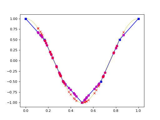
discretize.utils.interputils.interpmat(locs, x, y=None, z=None)

Local interpolation computed for each receiver point in turn

Parameters

• loc (numpy.ndarray) – Location of points to interpolate to

• x (numpy.ndarray) – Tensor of 1st dimension of grid.

• y (numpy.ndarray) – Tensor of 2nd dimension of grid. None by default.

• z (numpy.ndarray) – Tensor of 3rd dimension of grid. None by default.

Return type

scipy.sparse.csr_matrix

Returns

Interpolation matrix

(Source code, png, hires.png, pdf)

discretize.utils.interputils.volume_average(mesh_in, mesh_out, values=None, output=None)

Volume averaging interpolation between meshes.

This volume averaging function looks for overlapping cells in each mesh, and weights the output values by the partial volume ratio of the overlapping input cells. The volume average operation should result in an output such that np.sum(mesh_in.vol*values) = np.sum(mesh_out.vol*output), when the input and output meshes have the exact same extent. When the output mesh extent goes beyond the input mesh, it is assumed to have constant values in that direction. When the output mesh extent is smaller than the input mesh, only the overlapping extent of the input mesh contributes to the output.

This function operates in three different modes. If only mesh_in and mesh_out are given, the returned value is a scipy.sparse.csr_matrix that represents this operation (so it could potentially be applied repeatedly). If values is given, the volume averaging is performed right away (without internally forming the matrix) and the returned value is the result of this. If output is given as well, it will be filled with the values of the operation and then returned (assuming it has the correct dtype).

mesh_in: TensorMesh or TreeMesh

Input mesh (the mesh you are interpolating from)

mesh_out: TensorMesh or TreeMesh

Output mesh (the mesh you are interpolating to)

values: numpy.ndarray, optional

Array with values defined at the cells of mesh_in

output: numpy.ndarray, optional

Output array to be overwritten of length mesh_out.nC and type np.float64

scipy.sparse.csr_matrix or numpy.ndarray

If values is None, the returned value is a matrix representing this operation, otherwise it is a numpy.ndarray of the result of the operation.

Create two meshes with the same extent, but different divisions (the meshes do not have to be the same extent).

>>> import numpy as np
>>> from discretize import TensorMesh
>>> h1 = np.ones(32)
>>> h2 = np.ones(16)*2
>>> mesh_in = TensorMesh([h1, h1])
>>> mesh_out = TensorMesh([h2, h2])

Create a random model defined on the input mesh, and use volume averaging to interpolate it to the output mesh.

>>> from discretize.utils import volume_average
>>> model1 = np.random.rand(mesh_in.nC)
>>> model2 = volume_average(mesh_in, mesh_out, model1)

Because these two meshes’ cells are perfectly aligned, but the output mesh has 1 cell for each 4 of the input cells, this operation should effectively look like averaging each of those cells values

>>> import matplotlib.pyplot as plt
>>> plt.figure()
>>> ax1 = plt.subplot(121)
>>> mesh_in.plotImage(model1, ax=ax1)
>>> ax2 = plt.subplot(122)
>>> mesh_out.plotImage(model2, ax=ax2)
>>> plt.show()

Counter Utilities

class MyClass(object):
    def __init__(self, url):
        self.counter = Counter()

    @count
    def MyMethod(self):
        pass

    @timeIt
    def MySecondMethod(self):
        pass

c = MyClass('blah')
for i in range(100): c.MyMethod()
for i in range(300): c.MySecondMethod()
c.counter.summary()

Counters:
  MyClass.MyMethod                        :      100

Times:                                        mean      sum
  MyClass.MySecondMethod                  : 1.70e-06, 5.10e-04,  300x

The API

class SimPEG.utils.counter_utils.Counter

Counter allows anything that calls it to record iterations and timings in a simple way.

Also has plotting functions that allow quick recalls of data.

If you want to use this, import count or timeIt and use them as decorators on class methods.

class MyClass(object):
    def __init__(self, url):
        self.counter = Counter()

    @count
    def MyMethod(self):
        pass

    @timeIt
    def MySecondMethod(self):
        pass

c = MyClass('blah')
for i in range(100): c.MyMethod()
for i in range(300): c.MySecondMethod()
c.counter.summary()

count(prop)

Increases the count of the property.

countTic(prop)

Times a property call, this is the init call.

countToc(prop)

Times a property call, this is the end call.

summary()

Provides a text summary of the current counters and timers.

SimPEG.utils.counter_utils.count(f)

SimPEG.utils.counter_utils.timeIt(f)