2D inversion of Loop-Loop EM Data

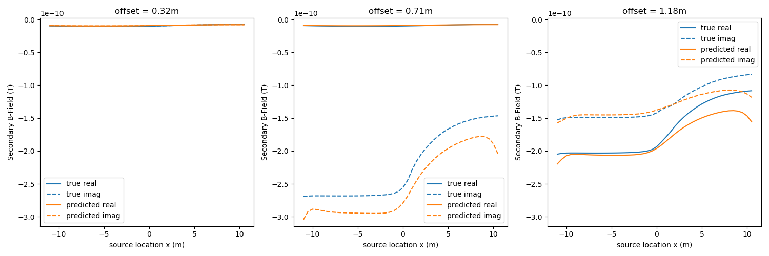
In this example, we consider a single line of loop-loop EM data at 30kHz with 3 different coil separations [0.32m, 0.71m, 1.18m]. We will use only Horizontal co-planar orientations (vertical magnetic dipole), and look at the real and imaginary parts of the secondary magnetic field.

We use the SimPEG.maps.Surject2Dto3D mapping to invert for a 2D model and perform the forward modelling in 3D.

import numpy as np
import matplotlib.pyplot as plt
import time
from pymatsolver import Pardiso as Solver

import discretize
from SimPEG import (
    maps,
    optimization,
    data_misfit,
    regularization,
    inverse_problem,
    inversion,
    directives,
    Report,
)
from SimPEG.electromagnetics import frequency_domain as FDEM

Setup

Define the survey and model parameters

sigma_surface = 10e-3
sigma_deep = 40e-3
sigma_air = 1e-8

coil_separations = [0.32, 0.71, 1.18]
freq = 30e3

print("skin_depth: {:1.2f}m".format(500 / np.sqrt(sigma_deep * freq)))

Out:

skin_depth: 14.43m

Define a dipping interface between the surface layer and the deeper layer

z_interface_shallow = -0.25
z_interface_deep = -1.5
x_dip = np.r_[0.0, 8.0]


def interface(x):
    interface = np.zeros_like(x)

    interface[x < x_dip[0]] = z_interface_shallow

    dipping_unit = (x >= x_dip[0]) & (x <= x_dip[1])
    x_dipping = (-(z_interface_shallow - z_interface_deep) / x_dip[1]) * (
        x[dipping_unit]
    ) + z_interface_shallow
    interface[dipping_unit] = x_dipping

    interface[x > x_dip[1]] = z_interface_deep

    return interface

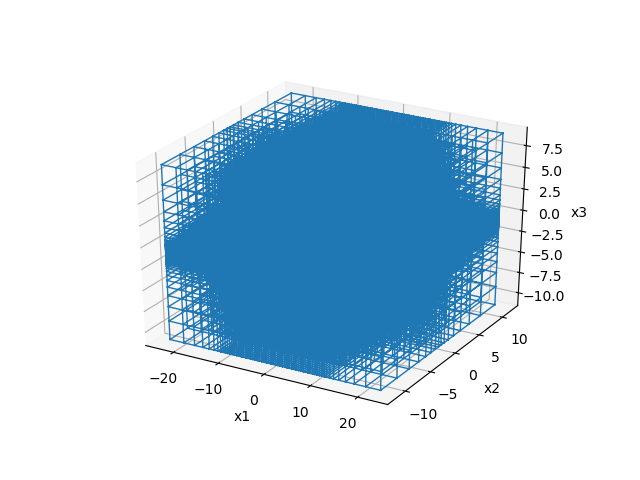
Forward Modelling Mesh

Here, we set up a 3D tensor mesh which we will perform the forward simulations on.

Note

In practice, a smaller horizontal discretization should be used to improve accuracy, particularly for the shortest offset (eg. you can try 0.25m).

csx = 0.5  # cell size for the horizontal direction
csz = 0.125  # cell size for the vertical direction
pf = 1.3  # expansion factor for the padding cells

npadx = 7  # number of padding cells in the x-direction
npady = 7  # number of padding cells in the y-direction
npadz = 11  # number of padding cells in the z-direction

core_domain_x = np.r_[-11.5, 11.5]  # extent of uniform cells in the x-direction
core_domain_z = np.r_[-2.0, 0.0]  # extent of uniform cells in the z-direction

# number of cells in the core region
ncx = int(np.diff(core_domain_x) / csx)
ncz = int(np.diff(core_domain_z) / csz)

# create a 3D tensor mesh
mesh = discretize.TensorMesh(
    [
        [(csx, npadx, -pf), (csx, ncx), (csx, npadx, pf)],
        [(csx, npady, -pf), (csx, 1), (csx, npady, pf)],
        [(csz, npadz, -pf), (csz, ncz), (csz, npadz, pf)],
    ]
)
# set the origin
mesh.x0 = np.r_[
    -mesh.hx.sum() / 2.0, -mesh.hy.sum() / 2.0, -mesh.hz[: npadz + ncz].sum()
]

print("the mesh has {} cells".format(mesh.nC))
mesh.plotGrid()

Out:

the mesh has 34200 cells

<matplotlib.axes._subplots.Axes3DSubplot object at 0x1845f99710>

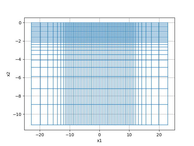
Inversion Mesh

Here, we set up a 2D tensor mesh which we will represent the inversion model on

inversion_mesh = discretize.TensorMesh([mesh.hx, mesh.hz[mesh.vectorCCz <= 0]])
inversion_mesh.x0 = [-inversion_mesh.hx.sum() / 2.0, -inversion_mesh.hy.sum()]
inversion_mesh.plotGrid()

Out:

<matplotlib.axes._subplots.AxesSubplot object at 0x1845f7ac50>

Mappings

Mappings are used to take the inversion model and represent it as electrical conductivity on the inversion mesh. We will invert for log-conductivity below the surface, fixing the conductivity of the air cells to 1e-8 S/m

# create a 2D mesh that includes air cells
mesh2D = discretize.TensorMesh([mesh.hx, mesh.hz], x0=mesh.x0[[0, 2]])
active_inds = mesh2D.gridCC[:, 1] < 0  # active indices are below the surface


mapping = (
    maps.Surject2Dto3D(mesh)
    * maps.InjectActiveCells(  # populates 3D space from a 2D model
        mesh2D, active_inds, sigma_air
    )
    * maps.ExpMap(  # adds air cells
        nP=inversion_mesh.nC
    )  # takes the exponential (log(sigma) --> sigma)
)

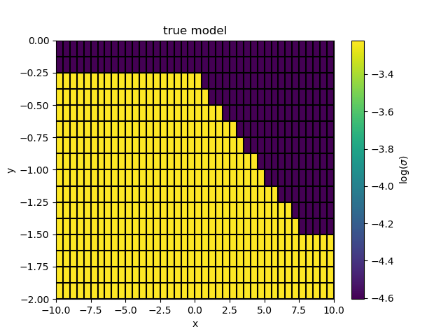
True Model

Create our true model which we will use to generate synthetic data for

m_true = np.log(sigma_deep) * np.ones(inversion_mesh.nC)
interface_depth = interface(inversion_mesh.gridCC[:, 0])
m_true[inversion_mesh.gridCC[:, 1] > interface_depth] = np.log(sigma_surface)

fig, ax = plt.subplots(1, 1)
cb = plt.colorbar(inversion_mesh.plotImage(m_true, ax=ax, grid=True)[0], ax=ax)
cb.set_label("$\log(\sigma)$")
ax.set_title("true model")
ax.set_xlim([-10, 10])
ax.set_ylim([-2, 0])

Out:

(-2, 0)

Survey

Create our true model which we will use to generate synthetic data for

src_locations = np.arange(-11, 11, 0.5)
src_z = 0.25  # src is 0.25m above the surface
orientation = "z"  # z-oriented dipole for horizontal co-planar loops

# reciever offset in 3D space
rx_offsets = np.vstack([np.r_[sep, 0.0, 0.0] for sep in coil_separations])

# create our source list - one source per location
srcList = []
for x in src_locations:
    src_loc = np.r_[x, 0.0, src_z]
    rx_locs = src_loc - rx_offsets

    rx_real = FDEM.Rx.PointMagneticFluxDensitySecondary(
        locations=rx_locs, orientation=orientation, component="real"
    )
    rx_imag = FDEM.Rx.PointMagneticFluxDensitySecondary(
        locations=rx_locs, orientation=orientation, component="imag"
    )

    src = FDEM.Src.MagDipole(
        receiver_list=[rx_real, rx_imag],
        loc=src_loc,
        orientation=orientation,
        freq=freq,
    )

    srcList.append(src)

# create the survey and problem objects for running the forward simulation
survey = FDEM.Survey(srcList)
prob = FDEM.Simulation3DMagneticFluxDensity(
    mesh, survey=survey, sigmaMap=mapping, Solver=Solver
)

Set up data for inversion

Generate clean, synthetic data. Later we will invert the clean data, and assign a standard deviation of 0.05, and a floor of 1e-11.

t = time.time()

data = prob.make_synthetic_data(
    m_true, relative_error=0.05, noise_floor=1e-11, add_noise=False
)

dclean = data.dclean
print("Done forward simulation. Elapsed time = {:1.2f} s".format(time.time() - t))


def plot_data(data, ax=None, color="C0", label=""):
    if ax is None:
        fig, ax = plt.subplots(1, 3, figsize=(15, 5))

    # data is [re, im, re, im, ...]
    data_real = data[0::2]
    data_imag = data[1::2]

    for i, offset in enumerate(coil_separations):
        ax[i].plot(
            src_locations,
            data_real[i :: len(coil_separations)],
            color=color,
            label="{} real".format(label),
        )
        ax[i].plot(
            src_locations,
            data_imag[i :: len(coil_separations)],
            "--",
            color=color,
            label="{} imag".format(label),
        )

        ax[i].set_title("offset = {:1.2f}m".format(offset))
        ax[i].legend()
        ax[i].grid(which="both")
        ax[i].set_ylim(np.r_[data.min(), data.max()] + 1e-11 * np.r_[-1, 1])

        ax[i].set_xlabel("source location x (m)")
        ax[i].set_ylabel("Secondary B-Field (T)")

    plt.tight_layout()
    return ax


ax = plot_data(dclean)

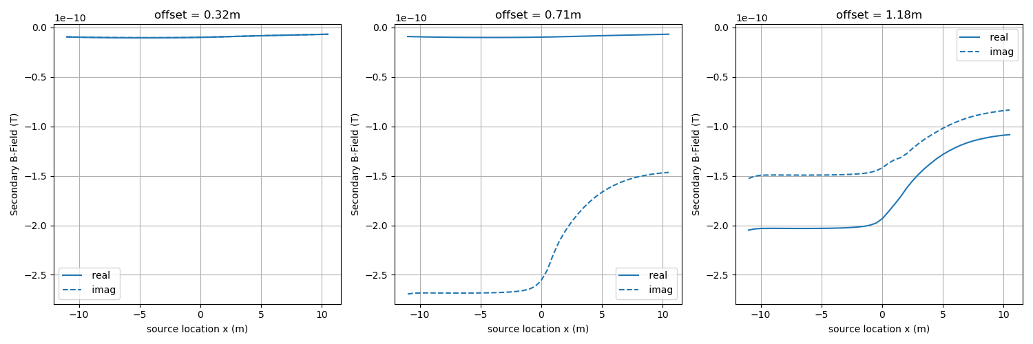
Out:

Done forward simulation. Elapsed time = 14.22 s

Set up the inversion

We create the data misfit, simple regularization (a Tikhonov-style regularization, SimPEG.regularization.Simple) The smoothness and smallness contributions can be set by including alpha_s, alpha_x, alpha_y as input arguments when the regularization is created. The default reference model in the regularization is the starting model. To set something different, you can input an mref into the regularization.

We estimate the trade-off parameter, beta, between the data misfit and regularization by the largest eigenvalue of the data misfit and the regularization. Here, we use a fixed beta, but could alternatively employ a beta-cooling schedule using SimPEG.directives.BetaSchedule

dmisfit = data_misfit.L2DataMisfit(simulation=prob, data=data)
reg = regularization.Simple(inversion_mesh)
opt = optimization.InexactGaussNewton(maxIterCG=10, remember="xc")
invProb = inverse_problem.BaseInvProblem(dmisfit, reg, opt)

betaest = directives.BetaEstimate_ByEig(beta0_ratio=0.25)
target = directives.TargetMisfit()

directiveList = [betaest, target]
inv = inversion.BaseInversion(invProb, directiveList=directiveList)

print("The target misfit is {:1.2f}".format(target.target))

Out:

The target misfit is 132.00

Run the inversion

We start from a half-space equal to the deep conductivity.

m0 = np.log(sigma_deep) * np.ones(inversion_mesh.nC)

t = time.time()
mrec = inv.run(m0)
print("\n Inversion Complete. Elapsed Time = {:1.2f} s".format(time.time() - t))

Out:

SimPEG.InvProblem will set Regularization.mref to m0.

        SimPEG.InvProblem is setting bfgsH0 to the inverse of the eval2Deriv.
        ***Done using same Solver and solverOpts as the problem***
model has any nan: 0
============================ Inexact Gauss Newton ============================
  #     beta     phi_d     phi_m       f      |proj(x-g)-x|  LS    Comment
-----------------------------------------------------------------------------
x0 has any nan: 0
   0  3.35e+00  3.66e+03  0.00e+00  3.66e+03    8.25e+02      0
   1  3.35e+00  4.48e+02  3.73e+01  5.73e+02    1.09e+02      0
------------------------- STOP! -------------------------
1 : |fc-fOld| = 0.0000e+00 <= tolF*(1+|f0|) = 3.6625e+02
1 : |xc-x_last| = 4.7159e+00 <= tolX*(1+|x0|) = 1.3056e+01
0 : |proj(x-g)-x|    = 1.0900e+02 <= tolG          = 1.0000e-01
0 : |proj(x-g)-x|    = 1.0900e+02 <= 1e3*eps       = 1.0000e-02
0 : maxIter   =      20    <= iter          =      2
------------------------- DONE! -------------------------

 Inversion Complete. Elapsed Time = 676.84 s

Plot the predicted and observed data

fig, ax = plt.subplots(1, 3, figsize=(15, 5))
plot_data(dclean, ax=ax, color="C0", label="true")
plot_data(invProb.dpred, ax=ax, color="C1", label="predicted")

Out:

array([<matplotlib.axes._subplots.AxesSubplot object at 0xd1cc62f60>,
       <matplotlib.axes._subplots.AxesSubplot object at 0xd1ccbba20>,
       <matplotlib.axes._subplots.AxesSubplot object at 0x18465a4b38>],
      dtype=object)

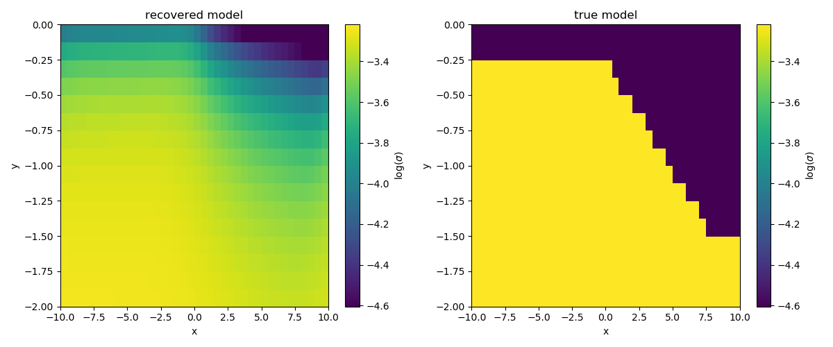
Plot the recovered model

fig, ax = plt.subplots(1, 2, figsize=(12, 5))

# put both plots on the same colorbar
clim = np.r_[np.log(sigma_surface), np.log(sigma_deep)]

# recovered model
cb = plt.colorbar(inversion_mesh.plotImage(mrec, ax=ax[0], clim=clim)[0], ax=ax[0],)
ax[0].set_title("recovered model")
cb.set_label("$\log(\sigma)$")

# true model
cb = plt.colorbar(inversion_mesh.plotImage(m_true, ax=ax[1], clim=clim)[0], ax=ax[1],)
ax[1].set_title("true model")
cb.set_label("$\log(\sigma)$")

# # uncomment to plot the true interface
# x = np.linspace(-10, 10, 50)
# [a.plot(x, interface(x), 'k') for a in ax]

[a.set_xlim([-10, 10]) for a in ax]
[a.set_ylim([-2, 0]) for a in ax]

plt.tight_layout()
plt.show()

Out:

/Users/josephcapriotti/codes/simpeg/examples/05-fdem/plot_inv_fdem_loop_loop_2Dinversion.py:344: UserWarning: Matplotlib is currently using agg, which is a non-GUI backend, so cannot show the figure.
  plt.show()

Print the version of SimPEG and dependencies

Report()

Tue May 26 19:08:58 2020 MDT
OS	Darwin	CPU(s)	8	Machine	x86_64
Architecture	64bit	Environment	Python
Python 3.6.10 |Anaconda, Inc.| (default, May 7 2020, 23:06:31) [GCC 4.2.1 Compatible Clang 4.0.1 (tags/RELEASE_401/final)]
SimPEG	0.14.0b2	discretize	0.4.11	pymatsolver	0.1.2
vectormath	0.2.2	properties	0.6.1	numpy	1.18.1
scipy	1.4.1	cython	0.29.17	IPython	7.13.0
matplotlib	3.1.3	ipywidgets	7.5.1
Intel(R) Math Kernel Library Version 2019.0.4 Product Build 20190411 for Intel(R) 64 architecture applications

Moving Forward

If you have suggestions for improving this example, please create a pull request on the example in SimPEG

You might try:

• improving the discretization

• changing beta

• changing the noise model

• playing with the regulariztion parameters

• …