\[\renewcommand{\div}{\nabla\cdot\,} \newcommand{\grad}{\vec \nabla} \newcommand{\curl}{{\vec \nabla}\times\,} \newcommand {\J}{{\vec J}} \renewcommand{\H}{{\vec H}} \newcommand {\E}{{\vec E}} \newcommand{\dcurl}{{\mathbf C}} \newcommand{\dgrad}{{\mathbf G}} \newcommand{\Acf}{{\mathbf A_c^f}} \newcommand{\Ace}{{\mathbf A_c^e}} \renewcommand{\S}{{\mathbf \Sigma}} \renewcommand{\Div}{{\mathbf {Div}}} \newcommand{\St}{{\mathbf \Sigma_\tau}} \newcommand{\T}{{\mathbf T}} \newcommand{\Tt}{{\mathbf T_\tau}} \newcommand{\diag}{\mathbf{diag}} \newcommand{\M}{{\mathbf M}} \newcommand{\MfMui}{{\M^f_{\mu^{-1}}}} \newcommand{\dMfMuI}{{d_m (\M^f_{\mu^{-1}})^{-1}}} \newcommand{\MeSig}{{\M^e_\sigma}} \newcommand{\MeSigInf}{{\M^e_{\sigma_\infty}}} \newcommand{\MeSigO}{{\M^e_{\sigma_0}}} \newcommand{\Me}{{\M^e}} \newcommand{\Mes}[1]{{\M^e_{#1}}} \newcommand{\Mee}{{\M^e_e}} \newcommand{\Mej}{{\M^e_j}} \newcommand{\BigO}[1]{\mathcal{O}\bigl(#1\bigr)} \newcommand{\bE}{\mathbf{E}} \newcommand{\bH}{\mathbf{H}} \newcommand{\B}{\vec{B}} \newcommand{\D}{\vec{D}} \renewcommand{\H}{\vec{H}} \newcommand{\s}{\vec{s}} \newcommand{\bfJ}{\bf{J}} \newcommand{\vecm}{\vec m} \renewcommand{\Re}{\mathsf{Re}} \renewcommand{\Im}{\mathsf{Im}} \renewcommand {\j} { {\vec j} } \newcommand {\h} { {\vec h} } \renewcommand {\b} { {\vec b} } \newcommand {\e} { {\vec e} } \newcommand {\c} { {\vec c} } \renewcommand {\d} { {\vec d} } \renewcommand {\u} { {\vec u} } \newcommand{\I}{\vec{I}}\]

Magnetics

The geomagnetic field can be ranked as the longest studied of all the geophysical properties of the earth. In addition, magnetic survey, has been used broadly in diverse realm e.g., mining, oil and gas industry and environmental engineering. Although, this geophysical application is quite common in geoscience; however, we do not have modular, well-documented and well-tested open-source codes, which perform forward and inverse problems of magnetic survey. Therefore, here we are going to build up magnetic forward and inverse modeling code based on two common methodologies for forward problem - differential equation and integral equation approaches.

First, we start with some backgrounds of magnetics, e.g., Maxwell’s equations. Based on that secondly, we use differential equation approach to solve forward problem with secondary field formulation. In order to discretzie our system here, we use finite volume approach with weak formulation. Third, we solve inverse problem through Gauss-Newton method.

Backgrounds

Maxwell’s equations for static case with out current source can be written as

\[ \begin{align}\begin{aligned}\begin{split}\nabla U = \frac{1}{\mu}\vec{B} \\\end{split}\\\nabla \cdot \vec{B} = 0\end{aligned}\end{align} \]

where \(\vec{B}\) is magnetic flux (\(T\)) and \(U\) is magnetic potential and \(\mu\) is permeability. Since we do not have any source term in above equations, boundary condition is going to be the driving force of our system as given below

\[(\vec{B}\cdot{\vec{n}})_{\partial\Omega} = B_{BC}\]

where \(\vec{n}\) means the unit normal vector on the boundary surface (\(\partial \Omega\)). By using seocondary field formulation we can rewrite above equations as

\[ \begin{align}\begin{aligned}\frac{1}{\mu}\vec{B}_s = (\frac{1}{\mu}_0-\frac{1}{\mu})\vec{B}_0+\nabla\phi_s\\\nabla \cdot \vec{B}_s = 0\\(\vec{B}_s\cdot{\vec{n}})_{\partial\Omega} = B_{sBC}\end{aligned}\end{align} \]

where \(\vec{B}_s\) is the secondary magnetic flux and \(\vec{B}_0\) is the background or primary magnetic flux. In practice, we consider our earth field, which we can get from International Geomagnetic Reference Field (IGRF) by specifying the time and location, as \(\vec{B}_0\). And based on this background fields, we compute secondary fields (\(\vec{B}_s\)). Now we introduce the susceptibility as

\[ \begin{align}\begin{aligned}\begin{split}\chi = \frac{\mu}{\mu_0} - 1 \\\end{split}\\\mu = \mu_0(1+\chi)\end{aligned}\end{align} \]

Since most materials in the earth have lower permeability than \(\mu_0\), usually \(\chi\) is greater than 0.

Note

Actually, this is an assumption, which means we are not sure exactly this is true, although we are sure, it is very rare that we can encounter those materials. Anyway, practical range of the susceptibility is \(0 < \chi < 1 \).

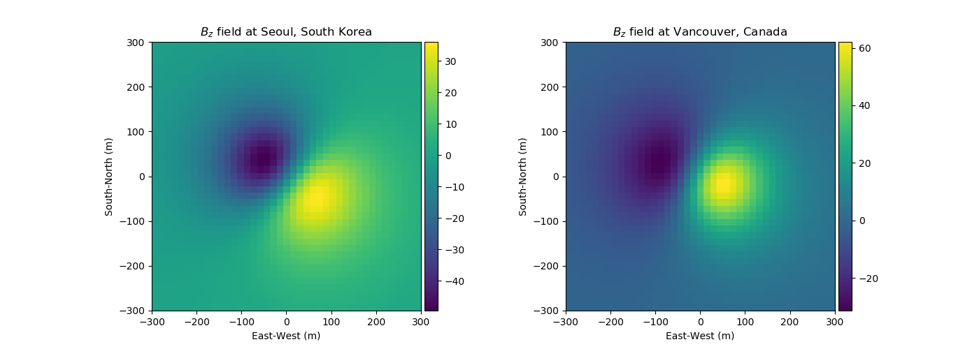
Since we compute secondary field based on the earth field, which can be different from different locations in the world, we can expect different anomalous responses in different locations in the earth. For instance, assume we have two susceptible spheres, which are exactly same. However, anomalous responses in Seoul and Vancouver are going to be different.

Since we can measure total fields ( \(\vec{B}\)), and usually have reasonably accurate earth field (\(\vec{B}_0\)), we can compute anomalous fields, \(\vec{B}_s\) from our observed data. If you want to download earth magnetic fields at specific location see this website (noaa).

What is our data?

In applied geophysics, which means in practice, it is common to refer to measurements as “the magnetic anomaly” and we can consider this as our observed data. For further descriptions in GPG materials for magnetic survey. Now we have the simple relation ship between “the magnetic anomaly” and the total field as

\[\triangle\vec{B} = |\hat{B}_o-\vec{B}_s|-|\hat{B}_o| \approx |\vec{B}_s|cos \theta\]

where \(\theta\) is the angle between total and anomalous fields, \(\hat{B}_o\) is the unit vector for \(\vec{B}_o\). Equivalently, we can use the vector dot product to show that the anomalous field is approximately equal to the projection of that field onto the direction of the inducing field. Using this approach we would write

\[\triangle\vec{B} = |\vec{B}_s|cos \theta = |\hat{B}_o||\vec{B}_s|cos \theta = \hat{B}_o \cdot \vec{B}_s\]

This is important because, in practice we usually use a total field magnetometer (like a proton precession or optically pumped sensor), which can measure only that part of the anomalous field which is in the direction of the earth’s main field.

Sphere in a whole space

Forward problem

Differential equation approach

\[ \begin{align}\begin{aligned}\mathbf{A}\mathbf{u} = \mathbf{rhs}\\\mathbf{A} = \Div(\MfMui)^{-1}\Div^{T}\\\mathbf{rhs} = \Div(\MfMui)^{-1}\mathbf{M}^f_{\mu_0^{-1}}\mathbf{B}_0 - \Div\mathbf{B}_0+\diag(v)\mathbf{D} \mathbf{P}_{out}^T \mathbf{B}_{sBC}\\\mathbf{B}_s = (\MfMui)^{-1}\mathbf{M}^f_{\mu_0^{-1}}\mathbf{B}_0-\mathbf{B}_0 -(\MfMui)^{-1}\Div^T \mathbf{u}\end{aligned}\end{align} \]

Mag Differential eq. approach

class SimPEG.potential_fields.magnetics.Simulation3DDifferential(*args, **kwargs)

Bases: SimPEG.simulation.BaseSimulation

Secondary field approach using differential equations!

Required Properties:

• counter (Counter): A SimPEG.utils.Counter object, an instance of Counter

• mesh (BaseMesh): a discretize mesh instance, an instance of BaseMesh

• sensitivity_path (String): path to store the sensitivty, a unicode string, Default: ./sensitivity/

• None

• solver_opts (Dictionary): solver options as a kwarg dict, a dictionary

• survey (Survey): a survey object, an instance of Survey

Optional Properties:

• model (Model): Inversion model., a numpy array of <class ‘float’>, <class ‘int’> with shape (*, *) or (*)

• mu (PhysicalProperty): Magnetic Permeability (H/m), a physical property, Default: 1.25663706212e-06

• muMap (Mapping): Mapping of Magnetic Permeability (H/m) to the inversion model., a SimPEG Map

• mui (PhysicalProperty): Inverse Magnetic Permeability (m/H), a physical property

• muiMap (Mapping): Mapping of Inverse Magnetic Permeability (m/H) to the inversion model., a SimPEG Map

Other Properties:

• muDeriv (Derivative): Derivative of Magnetic Permeability (H/m) wrt the model.

• muiDeriv (Derivative): Derivative of Inverse Magnetic Permeability (m/H) wrt the model.

property mu

Magnetic Permeability (H/m)

property muMap

Mapping of Magnetic Permeability (H/m) to the inversion model.

property muDeriv

Derivative of Magnetic Permeability (H/m) wrt the model.

property mui

Inverse Magnetic Permeability (m/H)

property muiMap

Mapping of Inverse Magnetic Permeability (m/H) to the inversion model.

property muiDeriv

Derivative of Inverse Magnetic Permeability (m/H) wrt the model.

property survey

survey (Survey): a survey object, an instance of Survey

property MfMuI

property MfMui

property MfMu0

makeMassMatrices(m)

getB0()

To use getB0 method, SimPEG requires that the survey be specified.

getRHS(m)

\[\mathbf{rhs} = \Div(\MfMui)^{-1}\mathbf{M}^f_{\mu_0^{-1}}\mathbf{B}_0 - \Div\mathbf{B}_0+\diag(v)\mathbf{D} \mathbf{P}_{out}^T \mathbf{B}_{sBC}\]

getA(m)

GetA creates and returns the A matrix for the Magnetics problem

The A matrix has the form:

\[\mathbf{A} = \Div(\MfMui)^{-1}\Div^{T}\]

fields(m)

Return magnetic potential (u) and flux (B) u: defined on the cell center [nC x 1] B: defined on the cell center [nG x 1]

After we compute u, then we update B.

\[\mathbf{B}_s = (\MfMui)^{-1}\mathbf{M}^f_{\mu_0^{-1}}\mathbf{B}_0-\mathbf{B}_0 -(\MfMui)^{-1}\Div^T \mathbf{u}\]

Jvec(m, v, u=None)

Computing Jacobian multiplied by vector

By setting our problem as

\[\mathbf{C}(\mathbf{m}, \mathbf{u}) = \mathbf{A}\mathbf{u} - \mathbf{rhs} = 0\]

And taking derivative w.r.t m

\[ \begin{align}\begin{aligned}\nabla \mathbf{C}(\mathbf{m}, \mathbf{u}) = \nabla_m \mathbf{C}(\mathbf{m}) \delta \mathbf{m} + \nabla_u \mathbf{C}(\mathbf{u}) \delta \mathbf{u} = 0\\\frac{\delta \mathbf{u}}{\delta \mathbf{m}} = - [\nabla_u \mathbf{C}(\mathbf{u})]^{-1}\nabla_m \mathbf{C}(\mathbf{m})\end{aligned}\end{align} \]

With some linear algebra we can have

\[ \begin{align}\begin{aligned}\nabla_u \mathbf{C}(\mathbf{u}) = \mathbf{A}\\\nabla_m \mathbf{C}(\mathbf{m}) = \frac{\partial \mathbf{A}}{\partial \mathbf{m}}(\mathbf{m})\mathbf{u} - \frac{\partial \mathbf{rhs}(\mathbf{m})}{\partial \mathbf{m}}\end{aligned}\end{align} \]

\[ \begin{align}\begin{aligned}\frac{\partial \mathbf{A}}{\partial \mathbf{m}}(\mathbf{m})\mathbf{u} = \frac{\partial \mathbf{\mu}}{\partial \mathbf{m}} \left[\Div \diag (\Div^T \mathbf{u}) \dMfMuI \right]\\\dMfMuI = \diag(\MfMui)^{-1}_{vec} \mathbf{Av}_{F2CC}^T\diag(\mathbf{v})\diag(\frac{1}{\mu^2})\\\frac{\partial \mathbf{rhs}(\mathbf{m})}{\partial \mathbf{m}} = \frac{\partial \mathbf{\mu}}{\partial \mathbf{m}} \left[ \Div \diag(\M^f_{\mu_{0}^{-1}}\mathbf{B}_0) \dMfMuI \right] - \diag(\mathbf{v})\mathbf{D} \mathbf{P}_{out}^T\frac{\partial B_{sBC}}{\partial \mathbf{m}}\end{aligned}\end{align} \]

In the end,

\[\frac{\delta \mathbf{u}}{\delta \mathbf{m}} = - [ \mathbf{A} ]^{-1}\left[ \frac{\partial \mathbf{A}}{\partial \mathbf{m}}(\mathbf{m})\mathbf{u} - \frac{\partial \mathbf{rhs}(\mathbf{m})}{\partial \mathbf{m}} \right]\]

A little tricky point here is we are not interested in potential (u), but interested in magnetic flux (B). Thus, we need sensitivity for B. Now we take derivative of B w.r.t m and have

\[ \begin{align}\begin{aligned}\frac{\delta \mathbf{B}} {\delta \mathbf{m}} = \frac{\partial \mathbf{\mu} } {\partial \mathbf{m} } \left[ \diag(\M^f_{\mu_{0}^{-1} } \mathbf{B}_0) \dMfMuI \ - \diag (\Div^T\mathbf{u})\dMfMuI \right ]\\ - (\MfMui)^{-1}\Div^T\frac{\delta\mathbf{u}}{\delta \mathbf{m}}\end{aligned}\end{align} \]

Finally we evaluate the above, but we should remember that

Note

We only want to evalute

\[\mathbf{J}\mathbf{v} = \frac{\delta \mathbf{P}\mathbf{B}} {\delta \mathbf{m}}\mathbf{v}\]

Since forming sensitivity matrix is very expensive in that this monster is “big” and “dense” matrix!!

Jtvec(m, v, u=None)

Computing Jacobian^T multiplied by vector.

\[ \begin{align}\begin{aligned}(\frac{\delta \mathbf{P}\mathbf{B}} {\delta \mathbf{m}})^{T} = \left[ \mathbf{P}_{deriv}\frac{\partial \mathbf{\mu} } {\partial \mathbf{m} } \left[ \diag(\M^f_{\mu_{0}^{-1} } \mathbf{B}_0) \dMfMuI \ - \diag (\Div^T\mathbf{u})\dMfMuI \right ]\right]^{T}\\ - \left[\mathbf{P}_{deriv}(\MfMui)^{-1}\Div^T\frac{\delta\mathbf{u}}{\delta \mathbf{m}} \right]^{T}\end{aligned}\end{align} \]

where

\[\mathbf{P}_{derv} = \frac{\partial \mathbf{P}}{\partial\mathbf{B}}\]

Note

Here we only want to compute

\[\mathbf{J}^{T}\mathbf{v} = (\frac{\delta \mathbf{P}\mathbf{B}} {\delta \mathbf{m}})^{T} \mathbf{v}\]

property Qfx

property Qfy

property Qfz

projectFields(u)

This function projects the fields onto the data space. Especially, here for we use total magnetic intensity (TMI) data, which is common in practice. First we project our B on to data location

\[\mathbf{B}_{rec} = \mathbf{P} \mathbf{B}\]

then we take the dot product between B and b_0

\[\text{TMI} = \vec{B}_s \cdot \hat{B}_0\]

projectFieldsDeriv(B)

This function projects the fields onto the data space.

\[\frac{\partial d_\text{pred}}{\partial \mathbf{B}} = \mathbf{P}\]

Especially, this function is for TMI data type

projectFieldsAsVector(B)

Jtvec_approx(m, v, f=None)

Approximate effect of transpose of J(m) on a vector v. :param numpy.ndarray m: model :param numpy.ndarray v: vector to multiply :param Fields f: fields :rtype: numpy.ndarray :return: JTv

Jvec_approx(m, v, f=None)

Approximate effect of J(m) on a vector v :param numpy.ndarray m: model :param numpy.ndarray v: vector to multiply :param Fields f: fields :rtype: numpy.ndarray :return: approxJv

property Solver

Solver has been deprecated. See simulation.solver for documentation

clean_on_model_update = []

property counter

counter (Counter): A SimPEG.utils.Counter object, an instance of Counter

deleteTheseOnModelUpdate = []

classmethod deserialize(value, trusted=False, strict=False, assert_valid=False, **kwargs)

Creates HasProperties instance from serialized dictionary

This uses the Property deserializers to deserialize all JSON-compatible dictionary values into their corresponding Property values on a new instance of a HasProperties class. Extra keys in the dictionary that do not correspond to Properties will be ignored.

Parameters:

• value - Dictionary to deserialize new instance from.

• trusted - If True (and if the input dictionary has '__class__' keyword and this class is in the registry), the new HasProperties class will come from the dictionary. If False (the default), only the HasProperties class this method is called on will be constructed.

• strict - Requires '__class__', if present on the input dictionary, to match the deserialized instance’s class. Also disallows unused properties in the input dictionary. Default is False.

• assert_valid - Require deserialized instance to be valid. Default is False.

• Any other keyword arguments will be passed through to the Property deserializers.

dpred(m, f=None)

Create the projected data from a model. The fields, f, (if provided) will be used for the predicted data instead of recalculating the fields (which may be expensive!).

\[d_\text{pred} = P(f(m))\]

Where P is a projection of the fields onto the data space.

equal(other)

Determine if two HasProperties instances are equivalent

Equivalence is determined by checking if all Property values on two instances are equal, using Property.equal.

make_synthetic_data(m, relative_error=0.05, noise_floor=0.0, f=None, add_noise=False, **kwargs)

Make synthetic data given a model, and a standard deviation. :param numpy.ndarray m: geophysical model :param numpy.ndarray relative_error: standard deviation :param numpy.ndarray noise_floor: noise floor :param numpy.ndarray f: fields for the given model (if pre-calculated)

property mesh

mesh (BaseMesh): a discretize mesh instance, an instance of BaseMesh

property model

model (Model): Inversion model., a numpy array of <class ‘float’>, <class ‘int’> with shape (*, *) or (*)

property needs_model

True if a model is necessary

pair(survey)

Deprecated pairing method. Please use simulation.survey=survey instead

residual(m, dobs, f=None)

The data residual:

\[\mu_\text{data} = \mathbf{d}_\text{pred} - \mathbf{d}_\text{obs}\]

Parameters

• m (numpy.ndarray) – geophysical model

• f (numpy.ndarray) – fields

Return type

numpy.ndarray

Returns

data residual

property sensitivity_path

sensitivity_path (String): path to store the sensitivty, a unicode string, Default: ./sensitivity/

serialize(include_class=True, save_dynamic=False, **kwargs)

Serializes a HasProperties instance to dictionary

This uses the Property serializers to serialize all Property values to a JSON-compatible dictionary. Properties that are undefined are not included. If the HasProperties instance contains a reference to itself, a properties.SelfReferenceError will be raised.

Parameters:

• include_class - If True (the default), the name of the class will also be saved to the serialized dictionary under key '__class__'

• save_dynamic - If True, dynamic properties are written to the serialized dict (default: False).

• Any other keyword arguments will be passed through to the Property serializers.

property solver

None

property solverOpts

solverOpts has been deprecated. See solver_opts for documentation

property solver_opts

solver_opts (Dictionary): solver options as a kwarg dict, a dictionary

summary()

validate()

Call all registered class validator methods

These are all methods decorated with @properties.validator. Validator methods are expected to raise a ValidationError if they fail.

Mag Integral eq. approach

class SimPEG.potential_fields.magnetics.Simulation3DIntegral(*args, **kwargs)

Bases: SimPEG.potential_fields.base.BasePFSimulation

magnetic simulation in integral form.

Required Properties:

• actInd (Array): Array of active cells (ground), a list or numpy array of <class ‘bool’>, <class ‘int’> with shape (*)

• counter (Counter): A SimPEG.utils.Counter object, an instance of Counter

• is_amplitude_data (Boolean): Whether the supplied data is amplitude data, a boolean, Default: False

• mesh (BaseMesh): a discretize mesh instance, an instance of BaseMesh

• modelType (StringChoice): Type of magnetization model, either “susceptibility” or “vector”, Default: susceptibility

• sensitivity_path (String): path to store the sensitivty, a unicode string, Default: ./sensitivity/

• None

• solver_opts (Dictionary): solver options as a kwarg dict, a dictionary

• store_sensitivities (StringChoice): Compute and store G, any of “disk”, “ram”, “forward_only”, Default: ram

• survey (BaseSurvey): a survey object, an instance of BaseSurvey

Optional Properties:

• chi (PhysicalProperty): Magnetic Susceptibility (SI), a physical property, Default: 1.0

• chiMap (Mapping): Mapping of Magnetic Susceptibility (SI) to the inversion model., a SimPEG Map

• linear_model (PhysicalProperty): The model for a linear problem, a physical property

• model (Model): Inversion model., a numpy array of <class ‘float’>, <class ‘int’> with shape (*, *) or (*)

• model_map (Mapping): Mapping of The model for a linear problem to the inversion model., a SimPEG Map

Other Properties:

• chiDeriv (Derivative): Derivative of Magnetic Susceptibility (SI) wrt the model.

• model_deriv (Derivative): Derivative of The model for a linear problem wrt the model.

property chi

Magnetic Susceptibility (SI)

property chiMap

Mapping of Magnetic Susceptibility (SI) to the inversion model.

property chiDeriv

Derivative of Magnetic Susceptibility (SI) wrt the model.

property modelType

modelType (StringChoice): Type of magnetization model, either “susceptibility” or “vector”, Default: susceptibility

property is_amplitude_data

is_amplitude_data (Boolean): Whether the supplied data is amplitude data, a boolean, Default: False

property M

M: ndarray

Magnetization matrix

fields(model)

u = fields(m) The field given the model. :param numpy.ndarray m: model :rtype: numpy.ndarray :return: u, the fields

property G

property nD

Number of data

property tmi_projection

getJtJdiag(m, W=None)

Return the diagonal of JtJ

Jvec(m, v, f=None)

Jv = Jvec(m, v, f=None) Effect of J(m) on a vector v. :param numpy.ndarray m: model :param numpy.ndarray v: vector to multiply :param Fields f: fields :rtype: numpy.ndarray :return: Jv

Jtvec(m, v, f=None)

Jtv = Jtvec(m, v, f=None) Effect of transpose of J(m) on a vector v. :param numpy.ndarray m: model :param numpy.ndarray v: vector to multiply :param Fields f: fields :rtype: numpy.ndarray :return: JTv

property fieldDeriv

classmethod normalized_fields(fields)

Return the normalized B fields

classmethod compute_amplitude(b_xyz)

Compute amplitude of the magnetic field

evaluate_integral(receiver_location, components)

Load in the active nodes of a tensor mesh and computes the magnetic forward relation between a cuboid and a given observation location outside the Earth [obsx, obsy, obsz]

INPUT: receiver_location: [obsx, obsy, obsz] nC x 3 Array

components: list[str]

List of magnetic components chosen from: ‘bx’, ‘by’, ‘bz’, ‘bxx’, ‘bxy’, ‘bxz’, ‘byy’, ‘byz’, ‘bzz’

OUTPUT: Tx = [Txx Txy Txz] Ty = [Tyx Tyy Tyz] Tz = [Tzx Tzy Tzz]

property deleteTheseOnModelUpdate

list() -> new empty list list(iterable) -> new list initialized from iterable’s items

property coordinate_system

Jtvec_approx(m, v, f=None)

Approximate effect of transpose of J(m) on a vector v. :param numpy.ndarray m: model :param numpy.ndarray v: vector to multiply :param Fields f: fields :rtype: numpy.ndarray :return: JTv

Jvec_approx(m, v, f=None)

Approximate effect of J(m) on a vector v :param numpy.ndarray m: model :param numpy.ndarray v: vector to multiply :param Fields f: fields :rtype: numpy.ndarray :return: approxJv

property Solver

Solver has been deprecated. See simulation.solver for documentation

property actInd

actInd (Array): Array of active cells (ground), a list or numpy array of <class ‘bool’>, <class ‘int’> with shape (*)

clean_on_model_update = []

property counter

counter (Counter): A SimPEG.utils.Counter object, an instance of Counter

classmethod deserialize(value, trusted=False, strict=False, assert_valid=False, **kwargs)

Creates HasProperties instance from serialized dictionary

This uses the Property deserializers to deserialize all JSON-compatible dictionary values into their corresponding Property values on a new instance of a HasProperties class. Extra keys in the dictionary that do not correspond to Properties will be ignored.

Parameters:

• value - Dictionary to deserialize new instance from.

• trusted - If True (and if the input dictionary has '__class__' keyword and this class is in the registry), the new HasProperties class will come from the dictionary. If False (the default), only the HasProperties class this method is called on will be constructed.

• strict - Requires '__class__', if present on the input dictionary, to match the deserialized instance’s class. Also disallows unused properties in the input dictionary. Default is False.

• assert_valid - Require deserialized instance to be valid. Default is False.

• Any other keyword arguments will be passed through to the Property deserializers.

dpred(m, f=None)

Create the projected data from a model. The fields, f, (if provided) will be used for the predicted data instead of recalculating the fields (which may be expensive!).

\[d_\text{pred} = P(f(m))\]

Where P is a projection of the fields onto the data space.

equal(other)

Determine if two HasProperties instances are equivalent

Equivalence is determined by checking if all Property values on two instances are equal, using Property.equal.

property forwardOnly

The forwardOnly property has been deprecated. Please set the store_sensitivites property instead. This will be removed in version 0.15.0 of SimPEG

getJ(m, f=None)

property linear_model

The model for a linear problem

linear_operator()

make_synthetic_data(m, relative_error=0.05, noise_floor=0.0, f=None, add_noise=False, **kwargs)

Make synthetic data given a model, and a standard deviation. :param numpy.ndarray m: geophysical model :param numpy.ndarray relative_error: standard deviation :param numpy.ndarray noise_floor: noise floor :param numpy.ndarray f: fields for the given model (if pre-calculated)

property mesh

mesh (BaseMesh): a discretize mesh instance, an instance of BaseMesh

property model

model (Model): Inversion model., a numpy array of <class ‘float’>, <class ‘int’> with shape (*, *) or (*)

property model_deriv

Derivative of The model for a linear problem wrt the model.

property model_map

Mapping of The model for a linear problem to the inversion model.

property n_cpu

The parallelized property has been removed. If interested, try out loading dask for parallelism by doing import SimPEG.dask. This will be removed in version 0.15.0 of SimPEG

property needs_model

True if a model is necessary

pair(survey)

Deprecated pairing method. Please use simulation.survey=survey instead

property parallelized

The parallelized property has been removed. If interested, try out loading dask for parallelism by doing import SimPEG.dask. This will be removed in version 0.15.0 of SimPEG

residual(m, dobs, f=None)

The data residual:

\[\mu_\text{data} = \mathbf{d}_\text{pred} - \mathbf{d}_\text{obs}\]

Parameters

• m (numpy.ndarray) – geophysical model

• f (numpy.ndarray) – fields

Return type

numpy.ndarray

Returns

data residual

property sensitivity_path

sensitivity_path (String): path to store the sensitivty, a unicode string, Default: ./sensitivity/

serialize(include_class=True, save_dynamic=False, **kwargs)

Serializes a HasProperties instance to dictionary

This uses the Property serializers to serialize all Property values to a JSON-compatible dictionary. Properties that are undefined are not included. If the HasProperties instance contains a reference to itself, a properties.SelfReferenceError will be raised.

Parameters:

• include_class - If True (the default), the name of the class will also be saved to the serialized dictionary under key '__class__'

• save_dynamic - If True, dynamic properties are written to the serialized dict (default: False).

• Any other keyword arguments will be passed through to the Property serializers.

property solver

None

property solverOpts

solverOpts has been deprecated. See solver_opts for documentation

property solver_opts

solver_opts (Dictionary): solver options as a kwarg dict, a dictionary

property store_sensitivities

store_sensitivities (StringChoice): Compute and store G, any of “disk”, “ram”, “forward_only”, Default: ram

summary()

property survey

survey (BaseSurvey): a survey object, an instance of BaseSurvey

validate()

Call all registered class validator methods

These are all methods decorated with @properties.validator. Validator methods are expected to raise a ValidationError if they fail.

Magnetics Survey

class SimPEG.potential_fields.magnetics.Survey(*args, **kwargs)

Bases: SimPEG.survey.BaseSurvey

Base Magnetics Survey

Required Properties:

• counter (Counter): A SimPEG counter object, an instance of Counter

• source_list (a list of BaseSrc): A list of sources for the survey, a list (each item is an instance of BaseSrc)

property components

property counter

counter (Counter): A SimPEG counter object, an instance of Counter

classmethod deserialize(value, trusted=False, strict=False, assert_valid=False, **kwargs)

Creates HasProperties instance from serialized dictionary

This uses the Property deserializers to deserialize all JSON-compatible dictionary values into their corresponding Property values on a new instance of a HasProperties class. Extra keys in the dictionary that do not correspond to Properties will be ignored.

Parameters:

• value - Dictionary to deserialize new instance from.

• trusted - If True (and if the input dictionary has '__class__' keyword and this class is in the registry), the new HasProperties class will come from the dictionary. If False (the default), only the HasProperties class this method is called on will be constructed.

• strict - Requires '__class__', if present on the input dictionary, to match the deserialized instance’s class. Also disallows unused properties in the input dictionary. Default is False.

• assert_valid - Require deserialized instance to be valid. Default is False.

• Any other keyword arguments will be passed through to the Property deserializers.

dpred(m=None, f=None)

equal(other)

Determine if two HasProperties instances are equivalent

Equivalence is determined by checking if all Property values on two instances are equal, using Property.equal.

eval(fields)

getSourceIndex(sources)

makeSyntheticData(m, std=None, f=None, force=False, **kwargs)

property nD

Number of data

property nRx

property nSrc

Number of Sources

pair(simulation)

property receiver_locations

serialize(include_class=True, save_dynamic=False, **kwargs)

Serializes a HasProperties instance to dictionary

This uses the Property serializers to serialize all Property values to a JSON-compatible dictionary. Properties that are undefined are not included. If the HasProperties instance contains a reference to itself, a properties.SelfReferenceError will be raised.

Parameters:

• include_class - If True (the default), the name of the class will also be saved to the serialized dictionary under key '__class__'

• save_dynamic - If True, dynamic properties are written to the serialized dict (default: False).

• Any other keyword arguments will be passed through to the Property serializers.

property source_list

source_list (a list of BaseSrc): A list of sources for the survey, a list (each item is an instance of BaseSrc)

property srcList

srcList has been deprecated. See source_list for documentation

validate()

Call all registered class validator methods

These are all methods decorated with @properties.validator. Validator methods are expected to raise a ValidationError if they fail.

property vnD

Vector number of data

Magnetics Source

class SimPEG.potential_fields.magnetics.SourceField(*args, **kwargs)

Bases: SimPEG.survey.BaseSrc

Define the inducing field

Required Properties:

• receiver_list (a list of BaseRx): receiver list, a list (each item is an instance of BaseRx)

Optional Properties:

• location (SourceLocationArray): Location of the source [x, y, z] in 3D, a 1D array denoting the source location of <class ‘float’>, <class ‘int’> with shape (*)

classmethod deserialize(value, trusted=False, strict=False, assert_valid=False, **kwargs)

Creates HasProperties instance from serialized dictionary

This uses the Property deserializers to deserialize all JSON-compatible dictionary values into their corresponding Property values on a new instance of a HasProperties class. Extra keys in the dictionary that do not correspond to Properties will be ignored.

Parameters:

• value - Dictionary to deserialize new instance from.

• trusted - If True (and if the input dictionary has '__class__' keyword and this class is in the registry), the new HasProperties class will come from the dictionary. If False (the default), only the HasProperties class this method is called on will be constructed.

• strict - Requires '__class__', if present on the input dictionary, to match the deserialized instance’s class. Also disallows unused properties in the input dictionary. Default is False.

• assert_valid - Require deserialized instance to be valid. Default is False.

• Any other keyword arguments will be passed through to the Property deserializers.

equal(other)

Determine if two HasProperties instances are equivalent

Equivalence is determined by checking if all Property values on two instances are equal, using Property.equal.

getReceiverIndex(receiver)

property loc

loc has been deprecated. See location for documentation

property location

location (SourceLocationArray): Location of the source [x, y, z] in 3D, a 1D array denoting the source location of <class ‘float’>, <class ‘int’> with shape (*)

property nD

Number of data

property receiver_list

receiver_list (a list of BaseRx): receiver list, a list (each item is an instance of BaseRx)

property rxList

rxList has been deprecated. See receiver_list for documentation

serialize(include_class=True, save_dynamic=False, **kwargs)

Serializes a HasProperties instance to dictionary

This uses the Property serializers to serialize all Property values to a JSON-compatible dictionary. Properties that are undefined are not included. If the HasProperties instance contains a reference to itself, a properties.SelfReferenceError will be raised.

Parameters:

• include_class - If True (the default), the name of the class will also be saved to the serialized dictionary under key '__class__'

• save_dynamic - If True, dynamic properties are written to the serialized dict (default: False).

• Any other keyword arguments will be passed through to the Property serializers.

validate()

Call all registered class validator methods

These are all methods decorated with @properties.validator. Validator methods are expected to raise a ValidationError if they fail.

property vnD

Vector number of data

Magnetics Source

class SimPEG.potential_fields.magnetics.Point(*args, **kwargs)

Bases: SimPEG.survey.BaseRx

Magnetic point receiver class for integral formulation

param numpy.ndarray locs

receiver locations index (ie. np.c_[ind_1, ind_2, ...])

param string component

receiver component “bxx”, “bxy”, “bxz”, “byy”, “byz”, “bzz”, “bx”, “by”, “bz”, “tmi” [default]

Required Properties:

• locations (RxLocationArray): Locations of the receivers (nRx x nDim), an array of receiver locations of <class ‘float’>, <class ‘int’> with shape (*, *)

• projGLoc (StringChoice): Projection grid location, default is CC, any of “CC”, “Fx”, “Fy”, “Fz”, “Ex”, “Ey”, “Ez”, “N”, Default: CC

• storeProjections (Boolean): Store calls to getP (organized by mesh), a boolean, Default: True

nD()

Number of data in the receiver.

receiver_index()

classmethod deserialize(value, trusted=False, strict=False, assert_valid=False, **kwargs)

Creates HasProperties instance from serialized dictionary

This uses the Property deserializers to deserialize all JSON-compatible dictionary values into their corresponding Property values on a new instance of a HasProperties class. Extra keys in the dictionary that do not correspond to Properties will be ignored.

Parameters:

• value - Dictionary to deserialize new instance from.

• trusted - If True (and if the input dictionary has '__class__' keyword and this class is in the registry), the new HasProperties class will come from the dictionary. If False (the default), only the HasProperties class this method is called on will be constructed.

• strict - Requires '__class__', if present on the input dictionary, to match the deserialized instance’s class. Also disallows unused properties in the input dictionary. Default is False.

• assert_valid - Require deserialized instance to be valid. Default is False.

• Any other keyword arguments will be passed through to the Property deserializers.

equal(other)

Determine if two HasProperties instances are equivalent

Equivalence is determined by checking if all Property values on two instances are equal, using Property.equal.

eval(**kwargs)

evalDeriv(**kwargs)

getP(mesh, projGLoc=None)

Returns the projection matrices as a list for all components collected by the receivers.

Note

Projection matrices are stored as a dictionary listed by meshes.

property locations

locations (RxLocationArray): Locations of the receivers (nRx x nDim), an array of receiver locations of <class ‘float’>, <class ‘int’> with shape (*, *)

property locs

locs has been deprecated. See locations for documentation

property projGLoc

projGLoc (StringChoice): Projection grid location, default is CC, any of “CC”, “Fx”, “Fy”, “Fz”, “Ex”, “Ey”, “Ez”, “N”, Default: CC

serialize(include_class=True, save_dynamic=False, **kwargs)

Serializes a HasProperties instance to dictionary

This uses the Property serializers to serialize all Property values to a JSON-compatible dictionary. Properties that are undefined are not included. If the HasProperties instance contains a reference to itself, a properties.SelfReferenceError will be raised.

Parameters:

• include_class - If True (the default), the name of the class will also be saved to the serialized dictionary under key '__class__'

• save_dynamic - If True, dynamic properties are written to the serialized dict (default: False).

• Any other keyword arguments will be passed through to the Property serializers.

property storeProjections

storeProjections (Boolean): Store calls to getP (organized by mesh), a boolean, Default: True

validate()

Call all registered class validator methods

These are all methods decorated with @properties.validator. Validator methods are expected to raise a ValidationError if they fail.

Mag analytic solutions

SimPEG.potential_fields.magnetics.analytics.MagSphereAnaFun(x, y, z, R, x0, y0, z0, mu1, mu2, H0, flag='total')

test Analytic function for Magnetics problem. The set up here is magnetic sphere in whole-space assuming that the inducing field is oriented in the x-direction.

• (x0, y0, z0)

• (x0, y0, z0 ): is the center location of sphere

• r: is the radius of the sphere

\[\mathbf{H}_0 = H_0\hat{x}\]

SimPEG.potential_fields.magnetics.analytics.CongruousMagBC(mesh, Bo, chi)

Computing boundary condition using Congrous sphere method. This is designed for secondary field formulation.

>> Input

• mesh: Mesh class

• Bo: np.array([Box, Boy, Boz]): Primary magnetic flux

• chi: susceptibility at cell volume

\[\vec{B}(r) = \frac{\mu_0}{4\pi} \frac{m}{ \| \vec{r} - \vec{r}_0\|^3}[3\hat{m}\cdot\hat{r}-\hat{m}]\]

SimPEG.potential_fields.magnetics.analytics.MagSphereAnaFunA(x, y, z, R, xc, yc, zc, chi, Bo, flag)

Computing boundary condition using Congrous sphere method. This is designed for secondary field formulation. >> Input mesh: Mesh class Bo: np.array([Box, Boy, Boz]): Primary magnetic flux Chi: susceptibility at cell volume

\[\vec{B}(r) = \frac{\mu_0}{4\pi}\frac{m}{\| \vec{r}-\vec{r}_0\|^3}[3\hat{m}\cdot\hat{r}-\hat{m}]\]

SimPEG.potential_fields.magnetics.analytics.IDTtoxyz(Inc, Dec, Btot)

Convert from Inclination, Declination, Total intensity of earth field to x, y, z

SimPEG.potential_fields.magnetics.analytics.MagSphereFreeSpace(x, y, z, R, xc, yc, zc, chi, Bo)

Computing the induced response of magnetic sphere in free-space.

>> Input x, y, z: Observation locations R: radius of the sphere xc, yc, zc: Location of the sphere chi: Susceptibility of sphere Bo: Inducing field components [bx, by, bz]*|H0|