Sparse Norm Inversion of Gravity Anomaly Data

Here we invert gravity anomaly data to recover a density contrast model. We formulate the inverse problem as an iteratively re-weighted least-squares (IRLS) optimization problem. For this tutorial, we focus on the following:

• Defining the survey from xyz formatted data

• Generating a mesh based on survey geometry

• Including surface topography

• Defining the inverse problem (data misfit, regularization, optimization)

• Specifying directives for the inversion

• Setting sparse and blocky norms

• Plotting the recovered model and data misfit

Although we consider gravity anomaly data in this tutorial, the same approach can be used to invert gradiometry and other types of geophysical data.

Import modules

import os
import numpy as np
import matplotlib as mpl
import matplotlib.pyplot as plt
import tarfile

from discretize import TensorMesh

from SimPEG.utils import plot2Ddata, surface2ind_topo
from SimPEG.potential_fields import gravity
from SimPEG import (
    maps,
    data,
    data_misfit,
    inverse_problem,
    regularization,
    optimization,
    directives,
    inversion,
    utils,
)

# sphinx_gallery_thumbnail_number = 3

Define File Names

File paths for assets we are loading. To set up the inversion, we require topography and field observations. The true model defined on the whole mesh is loaded to compare with the inversion result. These files are stored as a tar-file on our google cloud bucket: “https://storage.googleapis.com/simpeg/doc-assets/gravity.tar.gz”

# storage bucket where we have the data
data_source = "https://storage.googleapis.com/simpeg/doc-assets/gravity.tar.gz"

# download the data
downloaded_data = utils.download(data_source, overwrite=True)

# unzip the tarfile
tar = tarfile.open(downloaded_data, "r")
tar.extractall()
tar.close()

# path to the directory containing our data
dir_path = downloaded_data.split(".")[0] + os.path.sep

# files to work with
topo_filename = dir_path + "gravity_topo.txt"
data_filename = dir_path + "gravity_data.obs"
model_filename = dir_path + "true_model.txt"

Out:

overwriting /Users/josephcapriotti/codes/simpeg/tutorials/03-gravity/gravity.tar.gz
Downloading https://storage.googleapis.com/simpeg/doc-assets/gravity.tar.gz
   saved to: /Users/josephcapriotti/codes/simpeg/tutorials/03-gravity/gravity.tar.gz
Download completed!

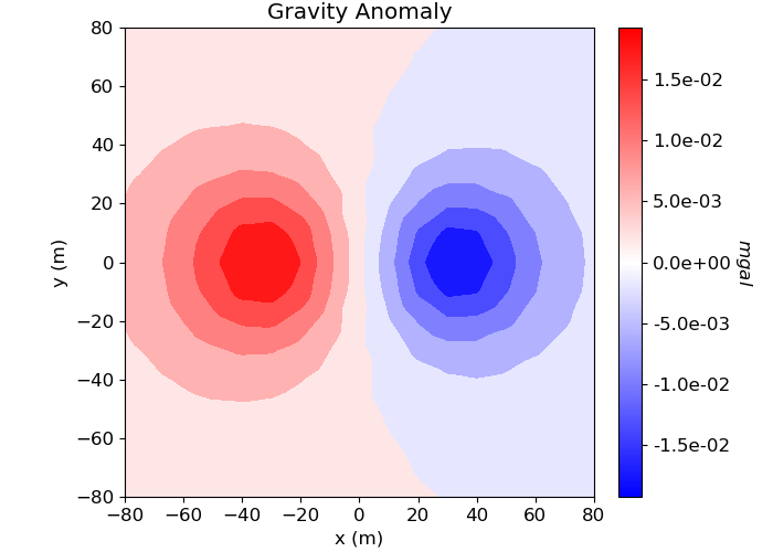
Load Data and Plot

Here we load and plot synthetic gravity anomaly data. Topography is generally defined as an (N, 3) array. Gravity data is generally defined with 4 columns: x, y, z and data.

# Load topography
xyz_topo = np.loadtxt(str(topo_filename))

# Load field data
dobs = np.loadtxt(str(data_filename))

# Define receiver locations and observed data
receiver_locations = dobs[:, 0:3]
dobs = dobs[:, -1]

# Plot
mpl.rcParams.update({"font.size": 12})
fig = plt.figure(figsize=(7, 5))

ax1 = fig.add_axes([0.1, 0.1, 0.73, 0.85])
plot2Ddata(receiver_locations, dobs, ax=ax1, contourOpts={"cmap": "bwr"})
ax1.set_title("Gravity Anomaly")
ax1.set_xlabel("x (m)")
ax1.set_ylabel("y (m)")

ax2 = fig.add_axes([0.8, 0.1, 0.03, 0.85])
norm = mpl.colors.Normalize(vmin=-np.max(np.abs(dobs)), vmax=np.max(np.abs(dobs)))
cbar = mpl.colorbar.ColorbarBase(
    ax2, norm=norm, orientation="vertical", cmap=mpl.cm.bwr, format="%.1e"
)
cbar.set_label("$mgal$", rotation=270, labelpad=15, size=12)

plt.show()

Out:

/Users/josephcapriotti/codes/simpeg/tutorials/03-gravity/plot_inv_1b_gravity_anomaly_irls.py:119: UserWarning: Matplotlib is currently using agg, which is a non-GUI backend, so cannot show the figure.
  plt.show()

Assign Uncertainties

Inversion with SimPEG requires that we define standard deviation on our data. This represents our estimate of the noise in our data. For gravity inversion, a constant floor value is generally applied to all data. For this tutorial, the standard deviation on each datum will be 1% of the maximum observed gravity anomaly value.

maximum_anomaly = np.max(np.abs(dobs))

uncertainties = 0.01 * maximum_anomaly * np.ones(np.shape(dobs))

Defining the Survey

Here, we define survey that will be used for this tutorial. Gravity surveys are simple to create. The user only needs an (N, 3) array to define the xyz locations of the observation locations. From this, the user can define the receivers and the source field.

# Define the receivers. The data consist of vertical gravity anomaly measurements.
# The set of receivers must be defined as a list.
receiver_list = gravity.receivers.Point(receiver_locations, components="gz")

receiver_list = [receiver_list]

# Define the source field
source_field = gravity.sources.SourceField(receiver_list=receiver_list)

# Define the survey
survey = gravity.survey.Survey(source_field)

Defining the Data

Here is where we define the data that are inverted. The data are defined by the survey, the observation values and the standard deviation.

data_object = data.Data(survey, dobs=dobs, standard_deviation=uncertainties)

Defining a Tensor Mesh

Here, we create the tensor mesh that will be used to invert gravity anomaly data. If desired, we could define an OcTree mesh.

dh = 5.0
hx = [(dh, 5, -1.3), (dh, 40), (dh, 5, 1.3)]
hy = [(dh, 5, -1.3), (dh, 40), (dh, 5, 1.3)]
hz = [(dh, 5, -1.3), (dh, 15)]
mesh = TensorMesh([hx, hy, hz], "CCN")

Starting/Reference Model and Mapping on Tensor Mesh

Here, we create starting and/or reference models for the inversion as well as the mapping from the model space to the active cells. Starting and reference models can be a constant background value or contain a-priori structures. Here, the background is 1e-6 g/cc.

# Define density contrast values for each unit in g/cc. Don't make this 0!
# Otherwise the gradient for the 1st iteration is zero and the inversion will
# not converge.
background_density = 1e-6

# Find the indecies of the active cells in forward model (ones below surface)
ind_active = surface2ind_topo(mesh, xyz_topo)

# Define mapping from model to active cells
nC = int(ind_active.sum())
model_map = maps.IdentityMap(nP=nC)  # model consists of a value for each active cell

# Define and plot starting model
starting_model = background_density * np.ones(nC)

Define the Physics

Here, we define the physics of the gravity problem by using the simulation class.

simulation = gravity.simulation.Simulation3DIntegral(
    survey=survey, mesh=mesh, rhoMap=model_map, actInd=ind_active
)

Define the Inverse Problem

The inverse problem is defined by 3 things:

1. Data Misfit: a measure of how well our recovered model explains the field data

2. Regularization: constraints placed on the recovered model and a priori information

3. Optimization: the numerical approach used to solve the inverse problem

# Define the data misfit. Here the data misfit is the L2 norm of the weighted
# residual between the observed data and the data predicted for a given model.
# Within the data misfit, the residual between predicted and observed data are
# normalized by the data's standard deviation.
dmis = data_misfit.L2DataMisfit(data=data_object, simulation=simulation)
dmis.W = utils.sdiag(1 / uncertainties)

# Define the regularization (model objective function).
reg = regularization.Sparse(mesh, indActive=ind_active, mapping=model_map)
reg.norms = np.c_[0, 2, 2, 2]

# Define how the optimization problem is solved. Here we will use a projected
# Gauss-Newton approach that employs the conjugate gradient solver.
opt = optimization.ProjectedGNCG(
    maxIter=100, lower=-1.0, upper=1.0, maxIterLS=20, maxIterCG=10, tolCG=1e-3
)

# Here we define the inverse problem that is to be solved
inv_prob = inverse_problem.BaseInvProblem(dmis, reg, opt)

Define Inversion Directives

Here we define any directiveas that are carried out during the inversion. This includes the cooling schedule for the trade-off parameter (beta), stopping criteria for the inversion and saving inversion results at each iteration.

# Defining a starting value for the trade-off parameter (beta) between the data
# misfit and the regularization.
starting_beta = directives.BetaEstimate_ByEig(beta0_ratio=1e-1)

# Defines the directives for the IRLS regularization. This includes setting
# the cooling schedule for the trade-off parameter.
update_IRLS = directives.Update_IRLS(
    f_min_change=1e-4, max_irls_iterations=30, coolEpsFact=1.5, beta_tol=1e-2,
)

# Defining the fractional decrease in beta and the number of Gauss-Newton solves
# for each beta value.
beta_schedule = directives.BetaSchedule(coolingFactor=5, coolingRate=1)

# Options for outputting recovered models and predicted data for each beta.
save_iteration = directives.SaveOutputEveryIteration(save_txt=False)

# Updating the preconditionner if it is model dependent.
update_jacobi = directives.UpdatePreconditioner()

# Add sensitivity weights
sensitivity_weights = directives.UpdateSensitivityWeights(everyIter=False)

# The directives are defined as a list.
directives_list = [
    update_IRLS,
    sensitivity_weights,
    starting_beta,
    beta_schedule,
    save_iteration,
    update_jacobi,
]

Running the Inversion

To define the inversion object, we need to define the inversion problem and the set of directives. We can then run the inversion.

# Here we combine the inverse problem and the set of directives
inv = inversion.BaseInversion(inv_prob, directives_list)

# Run inversion
recovered_model = inv.run(starting_model)

Out:

SimPEG.InvProblem will set Regularization.mref to m0.

        SimPEG.InvProblem is setting bfgsH0 to the inverse of the eval2Deriv.
        ***Done using same Solver and solverOpts as the problem***
model has any nan: 0
=============================== Projected GNCG ===============================
  #     beta     phi_d     phi_m       f      |proj(x-g)-x|  LS    Comment
-----------------------------------------------------------------------------
x0 has any nan: 0
   0  5.27e+05  1.33e+05  0.00e+00  1.33e+05    2.19e+02      0
   1  5.27e+04  1.40e+04  4.00e-02  1.61e+04    2.17e+02      0
   2  5.27e+03  7.91e+02  1.02e-01  1.33e+03    2.00e+02      0   Skip BFGS
Reached starting chifact with l2-norm regularization: Start IRLS steps...
eps_p: 0.059667753565190856 eps_q: 0.059667753565190856
   3  5.27e+02  6.34e+01  2.52e-01  1.96e+02    1.91e+02      0   Skip BFGS
   4  4.20e+02  2.41e+01  3.35e-01  1.65e+02    2.08e+02      0   Skip BFGS
   5  4.54e+02  1.64e+01  3.71e-01  1.85e+02    1.78e+02      0
   6  7.21e+02  1.04e+01  3.94e-01  2.94e+02    1.99e+02      0
   7  7.69e+02  1.67e+01  3.49e-01  2.85e+02    1.98e+02      0
   8  1.15e+03  1.12e+01  2.75e-01  3.27e+02    2.11e+02      0
   9  1.24e+03  1.64e+01  1.97e-01  2.62e+02    1.91e+02      0
  10  1.61e+03  1.32e+01  1.41e-01  2.41e+02    2.06e+02      0
  11  2.26e+03  1.20e+01  1.07e-01  2.53e+02    1.99e+02      0
  12  3.06e+03  1.25e+01  8.14e-02  2.62e+02    1.94e+02      0
  13  3.83e+03  1.38e+01  6.92e-02  2.79e+02    2.02e+02      0
  14  4.38e+03  1.53e+01  6.19e-02  2.86e+02    1.97e+02      0
  15  4.71e+03  1.65e+01  5.65e-02  2.82e+02    1.83e+02      0
  16  4.85e+03  1.74e+01  5.25e-02  2.72e+02    1.83e+02      0
  17  4.85e+03  1.81e+01  4.96e-02  2.58e+02    1.90e+02      0
  18  4.78e+03  1.84e+01  4.75e-02  2.45e+02    1.81e+02      0   Skip BFGS
  19  4.68e+03  1.85e+01  4.62e-02  2.35e+02    1.80e+02      0   Skip BFGS
  20  4.56e+03  1.87e+01  4.54e-02  2.26e+02    1.81e+02      0   Skip BFGS
  21  4.43e+03  1.88e+01  4.48e-02  2.17e+02    1.82e+02      0   Skip BFGS
  22  4.30e+03  1.87e+01  4.43e-02  2.09e+02    1.82e+02      0   Skip BFGS
  23  4.19e+03  1.86e+01  4.39e-02  2.03e+02    1.83e+02      0   Skip BFGS
  24  4.10e+03  1.86e+01  4.36e-02  1.97e+02    1.84e+02      0   Skip BFGS
  25  4.03e+03  1.85e+01  4.33e-02  1.93e+02    1.84e+02      0   Skip BFGS
  26  3.98e+03  1.83e+01  4.31e-02  1.90e+02    1.85e+02      0   Skip BFGS
  27  3.97e+03  1.82e+01  4.29e-02  1.88e+02    1.86e+02      0   Skip BFGS
  28  3.96e+03  1.81e+01  4.26e-02  1.87e+02    1.86e+02      0   Skip BFGS
  29  3.98e+03  1.80e+01  4.25e-02  1.87e+02    1.85e+02      0   Skip BFGS
  30  4.00e+03  1.79e+01  4.23e-02  1.87e+02    1.84e+02      0   Skip BFGS
  31  4.03e+03  1.79e+01  4.21e-02  1.88e+02    1.84e+02      0   Skip BFGS
  32  4.08e+03  1.78e+01  4.20e-02  1.89e+02    1.88e+02      0   Skip BFGS
Reach maximum number of IRLS cycles: 30
------------------------- STOP! -------------------------
1 : |fc-fOld| = 0.0000e+00 <= tolF*(1+|f0|) = 1.3312e+04
1 : |xc-x_last| = 1.4088e-02 <= tolX*(1+|x0|) = 1.0002e-01
0 : |proj(x-g)-x|    = 1.8775e+02 <= tolG          = 1.0000e-01
0 : |proj(x-g)-x|    = 1.8775e+02 <= 1e3*eps       = 1.0000e-02
0 : maxIter   =     100    <= iter          =     33
------------------------- DONE! -------------------------

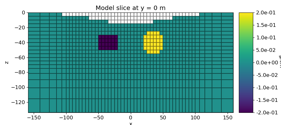
Plotting True Model and Recovered Model

# Load the true model (was defined on the whole mesh) and extract only the
# values on active cells.
true_model = np.loadtxt(str(model_filename))
true_model = true_model[ind_active]

# Plot True Model
fig = plt.figure(figsize=(9, 4))
plotting_map = maps.InjectActiveCells(mesh, ind_active, np.nan)

ax1 = fig.add_axes([0.1, 0.1, 0.73, 0.8])
mesh.plotSlice(
    plotting_map * true_model,
    normal="Y",
    ax=ax1,
    ind=int(mesh.nCy / 2),
    grid=True,
    clim=(np.min(true_model), np.max(true_model)),
    pcolorOpts={"cmap": "viridis"},
)
ax1.set_title("Model slice at y = 0 m")


ax2 = fig.add_axes([0.85, 0.1, 0.05, 0.8])
norm = mpl.colors.Normalize(vmin=np.min(true_model), vmax=np.max(true_model))
cbar = mpl.colorbar.ColorbarBase(
    ax2, norm=norm, orientation="vertical", cmap=mpl.cm.viridis, format="%.1e"
)
cbar.set_label("$g/cm^3$", rotation=270, labelpad=15, size=12)

plt.show()

# Plot Recovered Model
fig = plt.figure(figsize=(9, 4))
plotting_map = maps.InjectActiveCells(mesh, ind_active, np.nan)

ax1 = fig.add_axes([0.1, 0.1, 0.73, 0.8])
mesh.plotSlice(
    plotting_map * recovered_model,
    normal="Y",
    ax=ax1,
    ind=int(mesh.nCy / 2),
    grid=True,
    clim=(np.min(recovered_model), np.max(recovered_model)),
    pcolorOpts={"cmap": "viridis"},
)
ax1.set_title("Model slice at y = 0 m")

ax2 = fig.add_axes([0.85, 0.1, 0.05, 0.8])
norm = mpl.colors.Normalize(vmin=np.min(recovered_model), vmax=np.max(recovered_model))
cbar = mpl.colorbar.ColorbarBase(
    ax2, norm=norm, orientation="vertical", cmap=mpl.cm.viridis
)
cbar.set_label("$g/cm^3$", rotation=270, labelpad=15, size=12)

plt.show()

• 
• 

Out:

/Users/josephcapriotti/codes/simpeg/tutorials/03-gravity/plot_inv_1b_gravity_anomaly_irls.py:344: UserWarning: Matplotlib is currently using agg, which is a non-GUI backend, so cannot show the figure.
  plt.show()
/Users/josephcapriotti/codes/simpeg/tutorials/03-gravity/plot_inv_1b_gravity_anomaly_irls.py:369: UserWarning: Matplotlib is currently using agg, which is a non-GUI backend, so cannot show the figure.
  plt.show()

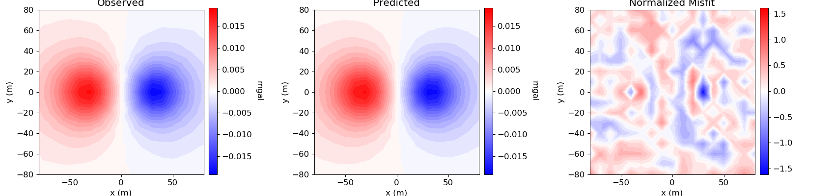
Plotting Predicted Data and Normalized Misfit

# Predicted data with final recovered model
dpred = inv_prob.dpred

# Observed data | Predicted data | Normalized data misfit
data_array = np.c_[dobs, dpred, (dobs - dpred) / uncertainties]

fig = plt.figure(figsize=(17, 4))
plot_title = ["Observed", "Predicted", "Normalized Misfit"]
plot_units = ["mgal", "mgal", ""]

ax1 = 3 * [None]
ax2 = 3 * [None]
norm = 3 * [None]
cbar = 3 * [None]
cplot = 3 * [None]
v_lim = [np.max(np.abs(dobs)), np.max(np.abs(dobs)), np.max(np.abs(data_array[:, 2]))]

for ii in range(0, 3):

    ax1[ii] = fig.add_axes([0.33 * ii + 0.03, 0.11, 0.23, 0.84])
    cplot[ii] = plot2Ddata(
        receiver_list[0].locations,
        data_array[:, ii],
        ax=ax1[ii],
        ncontour=30,
        clim=(-v_lim[ii], v_lim[ii]),
        contourOpts={"cmap": "bwr"},
    )
    ax1[ii].set_title(plot_title[ii])
    ax1[ii].set_xlabel("x (m)")
    ax1[ii].set_ylabel("y (m)")

    ax2[ii] = fig.add_axes([0.33 * ii + 0.25, 0.11, 0.01, 0.85])
    norm[ii] = mpl.colors.Normalize(vmin=-v_lim[ii], vmax=v_lim[ii])
    cbar[ii] = mpl.colorbar.ColorbarBase(
        ax2[ii], norm=norm[ii], orientation="vertical", cmap=mpl.cm.bwr
    )
    cbar[ii].set_label(plot_units[ii], rotation=270, labelpad=15, size=12)

plt.show()

Out:

/Users/josephcapriotti/codes/simpeg/tutorials/03-gravity/plot_inv_1b_gravity_anomaly_irls.py:415: UserWarning: Matplotlib is currently using agg, which is a non-GUI backend, so cannot show the figure.
  plt.show()