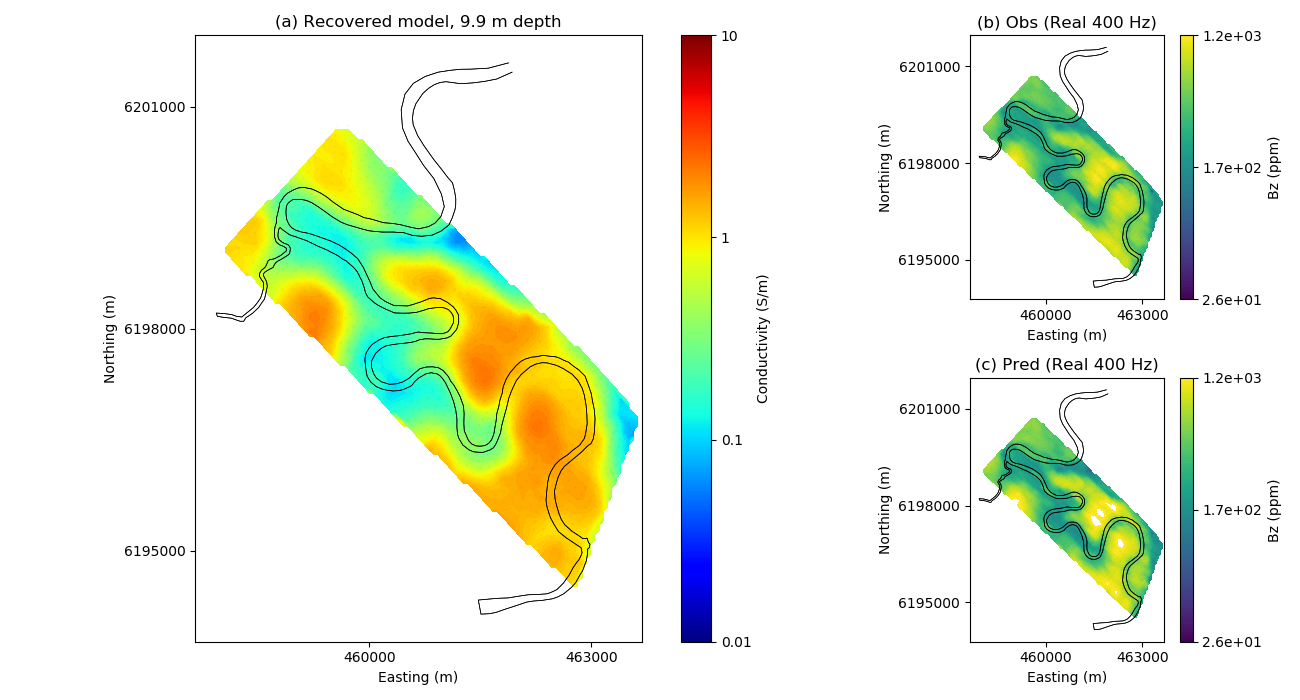
Heagy et al., 2017 1D RESOLVE Bookpurnong Inversion

In this example, perform a stitched 1D inversion of the Bookpurnong RESOLVE data. The original data can be downloaded from: https://storage.googleapis.com/simpeg/bookpurnong/bookpurnong.tar.gz

The forward simulation is performed on the cylindrically symmetric mesh using SimPEG.electromagnetics.frequency_domain.

Lindsey J. Heagy, Rowan Cockett, Seogi Kang, Gudni K. Rosenkjaer, Douglas W. Oldenburg, A framework for simulation and inversion in electromagnetics, Computers & Geosciences, Volume 107, 2017, Pages 1-19, ISSN 0098-3004, http://dx.doi.org/10.1016/j.cageo.2017.06.018.

The script and figures are also on figshare: https://doi.org/10.6084/m9.figshare.5107711

This example was updated for SimPEG 0.14.0 on January 31st, 2020 by Joseph Capriotti

Out:

Downloading https://storage.googleapis.com/simpeg/bookpurnong/bookpurnong_inversion.tar.gz
   saved to: /Users/josephcapriotti/codes/simpeg/examples/20-published/bookpurnong_inversion.tar.gz
Download completed!
-1186.8 223.6
25.71407326473829 1150.007175535807
/Users/josephcapriotti/codes/simpeg/examples/20-published/plot_booky_1Dstitched_resolve_inv.py:389: UserWarning: Matplotlib is currently using agg, which is a non-GUI backend, so cannot show the figure.
  plt.show()

import h5py
import tarfile
import os
import shutil
import numpy as np
import matplotlib.pyplot as plt

from pymatsolver import PardisoSolver
from scipy.constants import mu_0
from scipy.spatial import cKDTree

import discretize
from SimPEG import (
    maps,
    utils,
    data_misfit,
    regularization,
    optimization,
    inversion,
    inverse_problem,
    directives,
    data,
)
from SimPEG.electromagnetics import frequency_domain as FDEM


def download_and_unzip_data(
    url="https://storage.googleapis.com/simpeg/bookpurnong/bookpurnong_inversion.tar.gz",
):
    """
    Download the data from the storage bucket, unzip the tar file, return
    the directory where the data are
    """
    # download the data
    downloads = utils.download(url)

    # directory where the downloaded files are
    directory = downloads.split(".")[0]

    # unzip the tarfile
    tar = tarfile.open(downloads, "r")
    tar.extractall()
    tar.close()

    return downloads, directory


def resolve_1Dinversions(
    mesh,
    dobs,
    src_height,
    freqs,
    m0,
    mref,
    mapping,
    relative=0.08,
    floor=1e-14,
    rxOffset=7.86,
):
    """
    Perform a single 1D inversion for a RESOLVE sounding for Horizontal
    Coplanar Coil data (both real and imaginary).

    :param discretize.CylMesh mesh: mesh used for the forward simulation
    :param numpy.ndarray dobs: observed data
    :param float src_height: height of the source above the ground
    :param numpy.ndarray freqs: frequencies
    :param numpy.ndarray m0: starting model
    :param numpy.ndarray mref: reference model
    :param maps.IdentityMap mapping: mapping that maps the model to electrical conductivity
    :param float relative: percent error used to construct the data misfit term
    :param float floor: noise floor used to construct the data misfit term
    :param float rxOffset: offset between source and receiver.
    """

    # ------------------- Forward Simulation ------------------- #
    # set up the receivers
    bzr = FDEM.Rx.PointMagneticFluxDensitySecondary(
        np.array([[rxOffset, 0.0, src_height]]), orientation="z", component="real"
    )

    bzi = FDEM.Rx.PointMagneticFluxDensity(
        np.array([[rxOffset, 0.0, src_height]]), orientation="z", component="imag"
    )

    # source location
    srcLoc = np.array([0.0, 0.0, src_height])
    srcList = [
        FDEM.Src.MagDipole([bzr, bzi], freq, srcLoc, orientation="Z") for freq in freqs
    ]

    # construct a forward simulation
    survey = FDEM.Survey(srcList)
    prb = FDEM.Simulation3DMagneticFluxDensity(
        mesh, sigmaMap=mapping, Solver=PardisoSolver
    )
    prb.survey = survey

    # ------------------- Inversion ------------------- #
    # data misfit term
    uncert = abs(dobs) * relative + floor
    dat = data.Data(dobs=dobs, standard_deviation=uncert)
    dmisfit = data_misfit.L2DataMisfit(simulation=prb, data=dat)

    # regularization
    regMesh = discretize.TensorMesh([mesh.hz[mapping.maps[-1].indActive]])
    reg = regularization.Simple(regMesh)
    reg.mref = mref

    # optimization
    opt = optimization.InexactGaussNewton(maxIter=10)

    # statement of the inverse problem
    invProb = inverse_problem.BaseInvProblem(dmisfit, reg, opt)

    # Inversion directives and parameters
    target = directives.TargetMisfit()
    inv = inversion.BaseInversion(invProb, directiveList=[target])

    invProb.beta = 2.0  # Fix beta in the nonlinear iterations
    reg.alpha_s = 1e-3
    reg.alpha_x = 1.0
    prb.counter = opt.counter = utils.Counter()
    opt.LSshorten = 0.5
    opt.remember("xc")

    # run the inversion
    mopt = inv.run(m0)
    return mopt, invProb.dpred, survey.dobs


def run(runIt=False, plotIt=True, saveIt=False, saveFig=False, cleanup=True):
    """
    Run the bookpurnong 1D stitched RESOLVE inversions.

    :param bool runIt: re-run the inversions? Default downloads and plots saved results
    :param bool plotIt: show the plots?
    :param bool saveIt: save the re-inverted results?
    :param bool saveFig: save the figure
    :param bool cleanup: remove the downloaded results
    """

    # download the data
    downloads, directory = download_and_unzip_data()

    # Load resolve data
    resolve = h5py.File(os.path.sep.join([directory, "booky_resolve.hdf5"]), "r")

    river_path = resolve["river_path"][()]  # River path
    nSounding = resolve["data"].shape[0]  # the # of soundings

    # Bird height from surface
    b_height_resolve = resolve["src_elevation"][()]

    # fetch the frequencies we are considering
    cpi_inds = [0, 2, 6, 8, 10]  # Indices for HCP in-phase
    cpq_inds = [1, 3, 7, 9, 11]  # Indices for HCP quadrature
    frequency_cp = resolve["frequency_cp"][()]

    # build a mesh
    cs, ncx, ncz, npad = 1.0, 10.0, 10.0, 20
    hx = [(cs, ncx), (cs, npad, 1.3)]
    npad = 12
    temp = np.logspace(np.log10(1.0), np.log10(12.0), 19)
    temp_pad = temp[-1] * 1.3 ** np.arange(npad)
    hz = np.r_[temp_pad[::-1], temp[::-1], temp, temp_pad]
    mesh = discretize.CylMesh([hx, 1, hz], "00C")
    active = mesh.vectorCCz < 0.0

    # survey parameters
    rxOffset = 7.86  # tx-rx separation
    bp = -mu_0 / (4 * np.pi * rxOffset ** 3)  # primary magnetic field

    # re-run the inversion
    if runIt:

        # set up the mappings - we are inverting for 1D log conductivity
        # below the earth's surface.
        actMap = maps.InjectActiveCells(mesh, active, np.log(1e-8), nC=mesh.nCz)
        mapping = maps.ExpMap(mesh) * maps.SurjectVertical1D(mesh) * actMap

        # build starting and reference model
        sig_half = 1e-1
        sig_air = 1e-8
        sigma = np.ones(mesh.nCz) * sig_air
        sigma[active] = sig_half
        m0 = np.log(1e-1) * np.ones(active.sum())  # starting model
        mref = np.log(1e-1) * np.ones(active.sum())  # reference model

        # initalize empty lists for storing inversion results
        mopt_re = []  # recovered model
        dpred_re = []  # predicted data
        dobs_re = []  # observed data

        # downsample the data for the inversion
        nskip = 40

        # set up a noise model
        # 10% for the 3 lowest frequencies, 15% for the two highest
        relative = np.repeat(np.r_[np.ones(3) * 0.1, np.ones(2) * 0.15], 2)
        floor = abs(20 * bp * 1e-6)  # floor of 20ppm

        # loop over the soundings and invert each
        for rxind in range(nSounding):

            # convert data from ppm to magnetic field (A/m^2)
            dobs = (
                np.c_[
                    resolve["data"][rxind, :][cpi_inds].astype(float),
                    resolve["data"][rxind, :][cpq_inds].astype(float),
                ].flatten()
                * bp
                * 1e-6
            )

            # perform the inversion
            src_height = b_height_resolve[rxind].astype(float)
            mopt, dpred, dobs = resolve_1Dinversions(
                mesh,
                dobs,
                src_height,
                frequency_cp,
                m0,
                mref,
                mapping,
                relative=relative,
                floor=floor,
            )

            # add results to our list
            mopt_re.append(mopt)
            dpred_re.append(dpred)
            dobs_re.append(dobs)

        # save results
        mopt_re = np.vstack(mopt_re)
        dpred_re = np.vstack(dpred_re)
        dobs_re = np.vstack(dobs_re)

        if saveIt:
            np.save("mopt_re_final", mopt_re)
            np.save("dobs_re_final", dobs_re)
            np.save("dpred_re_final", dpred_re)

    mopt_re = resolve["mopt"][()]
    dobs_re = resolve["dobs"][()]
    dpred_re = resolve["dpred"][()]

    sigma = np.exp(mopt_re)
    indz = -7  # depth index

    # so that we can visually compare with literature (eg Viezzoli, 2010)
    cmap = "jet"

    # dummy figure for colobar
    fig = plt.figure()
    out = plt.scatter(np.ones(3), np.ones(3), c=np.linspace(-2, 1, 3), cmap=cmap)
    plt.close(fig)

    # plot from the paper
    fs = 13  # fontsize
    # matplotlib.rcParams['font.size'] = fs
    plt.figure(figsize=(13, 7))
    ax0 = plt.subplot2grid((2, 3), (0, 0), rowspan=2, colspan=2)
    ax1 = plt.subplot2grid((2, 3), (0, 2))
    ax2 = plt.subplot2grid((2, 3), (1, 2))

    # titles of plots
    title = [
        ("(a) Recovered model, %.1f m depth") % (-mesh.vectorCCz[active][indz]),
        "(b) Obs (Real 400 Hz)",
        "(c) Pred (Real 400 Hz)",
    ]

    temp = sigma[:, indz]
    tree = cKDTree(list(zip(resolve["xy"][:, 0], resolve["xy"][:, 1])))
    d, d_inds = tree.query(list(zip(resolve["xy"][:, 0], resolve["xy"][:, 1])), k=20)
    w = 1.0 / (d + 100.0) ** 2.0
    w = utils.sdiag(1.0 / np.sum(w, axis=1)) * (w)
    xy = resolve["xy"]
    temp = (temp.flatten()[d_inds] * w).sum(axis=1)
    utils.plot2Ddata(
        xy,
        temp,
        ncontour=100,
        scale="log",
        dataloc=False,
        contourOpts={"cmap": cmap, "vmin": 1e-2, "vmax": 1e1},
        ax=ax0,
    )
    ax0.plot(resolve["xy"][:, 0], resolve["xy"][:, 1], "k.", alpha=0.02, ms=1)

    cb = plt.colorbar(out, ax=ax0, ticks=np.linspace(-2, 1, 4), format="$10^{%.1f}$")
    cb.set_ticklabels(["0.01", "0.1", "1", "10"])
    cb.set_label("Conductivity (S/m)")
    ax0.plot(river_path[:, 0], river_path[:, 1], "k-", lw=0.5)

    # plot observed and predicted data
    freq_ind = 0
    axs = [ax1, ax2]
    temp_dobs = dobs_re[:, freq_ind].copy()
    ax1.plot(river_path[:, 0], river_path[:, 1], "k-", lw=0.5)
    inf = temp_dobs / abs(bp) * 1e6
    print(inf.min(), inf.max())
    out = utils.plot2Ddata(
        resolve["xy"][()],
        temp_dobs / abs(bp) * 1e6,
        ncontour=100,
        scale="log",
        dataloc=False,
        ax=ax1,
        contourOpts={"cmap": "viridis"},
    )
    vmin, vmax = out[0].get_clim()
    print(vmin, vmax)
    cb = plt.colorbar(
        out[0],
        ticks=np.logspace(np.log10(vmin), np.log10(vmax), 3),
        ax=ax1,
        format="%.1e",
        fraction=0.046,
        pad=0.04,
    )
    cb.set_label("Bz (ppm)")
    temp_dpred = dpred_re[:, freq_ind].copy()
    # temp_dpred[mask_:_data] = np.nan
    ax2.plot(river_path[:, 0], river_path[:, 1], "k-", lw=0.5)
    utils.plot2Ddata(
        resolve["xy"][()],
        temp_dpred / abs(bp) * 1e6,
        ncontour=100,
        scale="log",
        dataloc=False,
        contourOpts={"vmin": vmin, "vmax": vmax, "cmap": "viridis"},
        ax=ax2,
    )
    cb = plt.colorbar(
        out[0],
        ticks=np.logspace(np.log10(vmin), np.log10(vmax), 3),
        ax=ax2,
        format="%.1e",
        fraction=0.046,
        pad=0.04,
    )
    cb.set_label("Bz (ppm)")

    for i, ax in enumerate([ax0, ax1, ax2]):
        xticks = [460000, 463000]
        yticks = [6195000, 6198000, 6201000]
        xloc, yloc = 462100.0, 6196500.0
        ax.set_xticks(xticks)
        ax.set_yticks(yticks)
        # ax.plot(xloc, yloc, 'wo')
        ax.plot(river_path[:, 0], river_path[:, 1], "k", lw=0.5)

        ax.set_aspect("equal")
        ax.plot(resolve["xy"][:, 0], resolve["xy"][:, 1], "k.", alpha=0.02, ms=1)

        ax.set_yticklabels([str(f) for f in yticks])
        ax.set_ylabel("Northing (m)")
        ax.set_xlabel("Easting (m)")
        ax.set_title(title[i])

    plt.tight_layout()

    if plotIt:
        plt.show()

    if saveFig is True:
        fig.savefig("obspred_resolve.png", dpi=200)

    resolve.close()
    if cleanup:
        os.remove(downloads)
        shutil.rmtree(directory)


if __name__ == "__main__":
    run(runIt=False, plotIt=True, saveIt=True, saveFig=False, cleanup=True)