Effective Medium Theory Mapping¶

This example uses Self Consistent Effective Medium Theory to estimate the electrical conductivity of a mixture of two phases of materials. Given the electrical conductivity of each of the phases (\(\sigma_0\), \(\sigma_1\)), the SimPEG.maps.SelfConsistentEffectiveMedium map takes the concentration of phase-1 (\(\phi_1\)) and maps this to an electrical conductivity.

This mapping is used in chapter 2 of:

Heagy, Lindsey J.(2018, in prep) Electromagnetic methods for imaging subsurface injections. University of British Columbia

author: @lheagy

import numpy as np
import matplotlib.pyplot as plt
from SimPEG import maps
from matplotlib import rcParams

rcParams["font.size"] = 12

Conductivities¶

Here we consider a mixture composed of fluid (3 S/m) and conductive particles which we will vary the conductivity of.

sigma_fluid = 3
sigma1 = np.logspace(1, 5, 5)  # look at a range of particle conductivities
phi = np.linspace(0.0, 1, 1000)  # vary the volume of particles

Construct the Mapping¶

We set the conductivity of the phase-0 material to the conductivity of the fluid. The mapping will then take a concentration (by volume), of phase-1 material and compute the effective conductivity

scemt = maps.SelfConsistentEffectiveMedium(sigma0=sigma_fluid, sigma1=1)

Loop over a range of particle conductivities¶

We loop over the values defined as sigma1 and compute the effective conductivity of the mixture for each concentration in the phi vector

sige = np.zeros([phi.size, sigma1.size])

for i, s in enumerate(sigma1):
    scemt.sigma1 = s
    sige[:, i] = scemt * phi

Out:

/Users/josephcapriotti/opt/anaconda3/envs/py36/lib/python3.6/site-packages/SimPEG/maps.py:998: UserWarning: Maximum number of iterations reached
  warnings.warn("Maximum number of iterations reached")

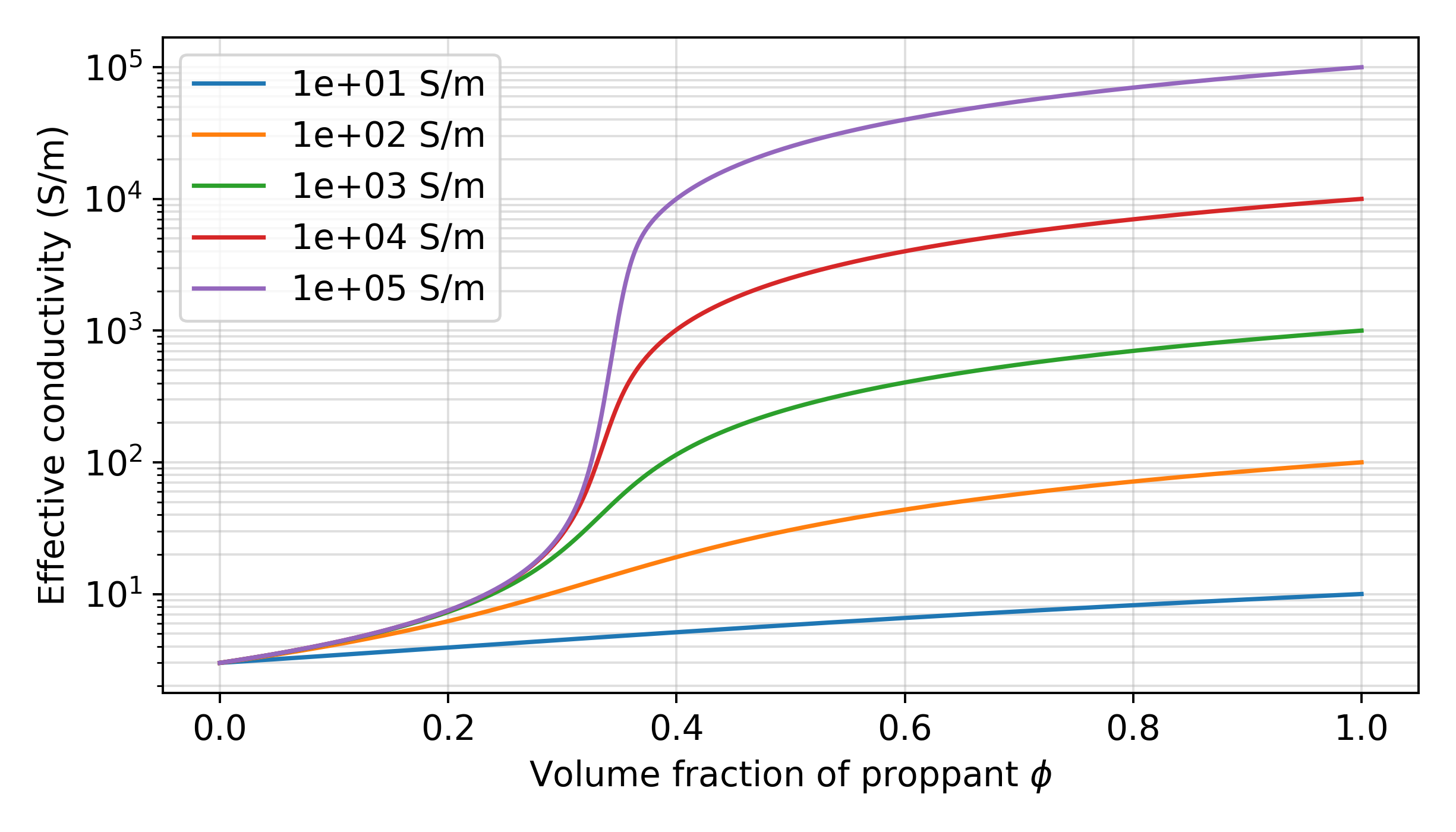
Plot the effective conductivity¶

The plot shows the effective conductivity of 5 difference mixtures. In all cases, the conductivity of the fluid, \(\sigma_0\), is 3 S/m. The conductivity of the particles is indicated in the legend

fig, ax = plt.subplots(1, 1, figsize=(7, 4), dpi=350)

ax.semilogy(phi, sige)
ax.grid(which="both", alpha=0.4)
ax.legend(["{:1.0e} S/m".format(s) for s in sigma1])
ax.set_xlabel("Volume fraction of proppant $\phi$")
ax.set_ylabel("Effective conductivity (S/m)")

plt.tight_layout()