Straight Ray with Volume Data Misfit Term

Based on the SEG abstract Heagy, Cockett and Oldenburg, 2014.

Heagy, L. J., Cockett, A. R., & Oldenburg, D. W. (2014, August 5). Parametrized Inversion Framework for Proppant Volume in a Hydraulically Fractured Reservoir. SEG Technical Program Expanded Abstracts 2014. Society of Exploration Geophysicists. doi:10.1190/segam2014-1639.1

This example is a simple joint inversion that consists of a

• data misfit for the tomography problem

• data misfit for the volume of the inclusions (uses the effective medium theory mapping)

• model regularization

• 
• 
• 
• 

Out:

True Volume: 0.026000000000000006
SimPEG.InvProblem will set Regularization.mref to m0.

        SimPEG.InvProblem is setting bfgsH0 to the inverse of the eval2Deriv.
        ***Done using same Solver and solverOpts as the problem***
model has any nan: 0
=============================== Projected GNCG ===============================
  #     beta     phi_d     phi_m       f      |proj(x-g)-x|  LS    Comment
-----------------------------------------------------------------------------
x0 has any nan: 0
   0  2.50e-01  6.52e+03  0.00e+00  6.52e+03    3.22e+01      0
/Users/josephcapriotti/opt/anaconda3/envs/py36/lib/python3.6/site-packages/SimPEG/maps.py:998: UserWarning: Maximum number of iterations reached
  warnings.warn("Maximum number of iterations reached")
   1  2.50e-01  1.10e+03  6.48e-01  1.10e+03    5.26e+00      1
   2  2.50e-01  3.85e+02  6.37e-01  3.86e+02    1.07e+01      0
------------------------------------------------------------------
0 :    ft     = 3.8628e+02 <= alp*descent     = 3.8550e+02
1 : maxIterLS =      10    <= iterLS          =     10
------------------------- End Linesearch -------------------------
The linesearch got broken. Boo.

Total recovered volume (no vol misfit term in inversion): 0.00011792090275769777

        SimPEG.InvProblem is setting bfgsH0 to the inverse of the eval2Deriv.
        ***Done using same Solver and solver_opts as the Simulation2DIntegral problem***
model has any nan: 0
=============================== Projected GNCG ===============================
  #     beta     phi_d     phi_m       f      |proj(x-g)-x|  LS    Comment
-----------------------------------------------------------------------------
x0 has any nan: 0
   0  2.50e-01  6.55e+03  0.00e+00  6.55e+03    3.10e+01      0
   1  2.50e-01  8.47e+02  6.15e-01  8.47e+02    1.37e+01      1
   2  2.50e-01  3.86e+02  6.14e-01  3.86e+02    1.65e+01      0
------------------------------------------------------------------
0 :    ft     = 3.8635e+02 <= alp*descent     = 3.8618e+02
1 : maxIterLS =      10    <= iterLS          =     10
------------------------- End Linesearch -------------------------
The linesearch got broken. Boo.

Total volume (vol misfit term in inversion): 0.00012051199854621248
/Users/josephcapriotti/opt/anaconda3/envs/py36/lib/python3.6/site-packages/SimPEG/maps.py:998: UserWarning: Maximum number of iterations reached
  warnings.warn("Maximum number of iterations reached")
/Users/josephcapriotti/opt/anaconda3/envs/py36/lib/python3.6/site-packages/SimPEG/maps.py:998: UserWarning: Maximum number of iterations reached
  warnings.warn("Maximum number of iterations reached")
/Users/josephcapriotti/codes/simpeg/examples/20-published/plot_tomo_joint_with_volume.py:190: MatplotlibDeprecationWarning:
The set_clim function was deprecated in Matplotlib 3.1 and will be removed in 3.3. Use ScalarMappable.set_clim instead.
  cb.set_clim([0.0, phi1])
/Users/josephcapriotti/codes/simpeg/examples/20-published/plot_tomo_joint_with_volume.py:205: UserWarning: Matplotlib is currently using agg, which is a non-GUI backend, so cannot show the figure.
  plt.show()

import numpy as np
import scipy.sparse as sp
import properties
import matplotlib.pyplot as plt

from SimPEG.seismic import straight_ray_tomography as tomo
import discretize
from SimPEG import (
    maps,
    utils,
    regularization,
    optimization,
    inverse_problem,
    inversion,
    data_misfit,
    directives,
    objective_function,
)


class Volume(objective_function.BaseObjectiveFunction):

    """
    A regularization on the volume integral of the model

    .. math::

        \phi_v = \frac{1}{2}|| \int_V m dV - \text{knownVolume} ||^2
    """

    knownVolume = properties.Float("known volume", default=0.0, min=0.0)

    def __init__(self, mesh, **kwargs):
        self.mesh = mesh
        super(Volume, self).__init__(**kwargs)

    def __call__(self, m):
        return 0.5 * (self.estVol(m) - self.knownVolume) ** 2

    def estVol(self, m):
        return np.inner(self.mesh.vol, m)

    def deriv(self, m):
        # return (self.mesh.vol * np.inner(self.mesh.vol, m))
        return self.mesh.vol * (self.knownVolume - np.inner(self.mesh.vol, m))

    def deriv2(self, m, v=None):
        if v is not None:
            return utils.mkvc(self.mesh.vol * np.inner(self.mesh.vol, v))
        else:
            # TODO: this is inefficent. It is a fully dense matrix
            return sp.csc_matrix(np.outer(self.mesh.vol, self.mesh.vol))


def run(plotIt=True):

    nC = 40
    de = 1.0
    h = np.ones(nC) * de / nC
    M = discretize.TensorMesh([h, h])

    y = np.linspace(M.vectorCCy[0], M.vectorCCx[-1], int(np.floor(nC / 4)))
    rlocs = np.c_[0 * y + M.vectorCCx[-1], y]
    rx = tomo.Rx(rlocs)

    srcList = [
        tomo.Src(location=np.r_[M.vectorCCx[0], yi], receiver_list=[rx]) for yi in y
    ]

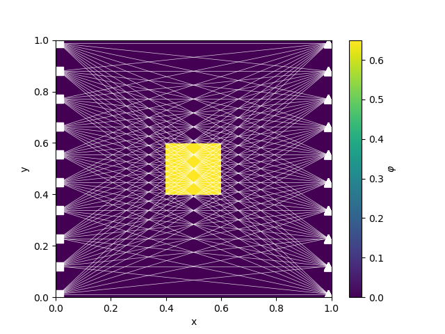
    # phi model
    phi0 = 0
    phi1 = 0.65
    phitrue = utils.model_builder.defineBlock(
        M.gridCC, [0.4, 0.6], [0.6, 0.4], [phi1, phi0]
    )

    knownVolume = np.sum(phitrue * M.vol)
    print("True Volume: {}".format(knownVolume))

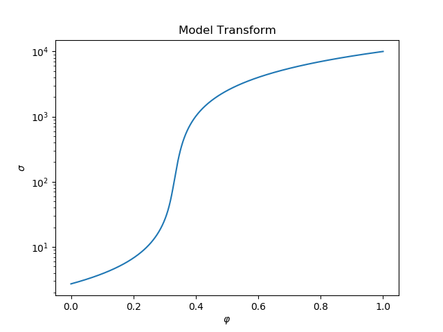
    # Set up true conductivity model and plot the model transform
    sigma0 = np.exp(1)
    sigma1 = 1e4

    if plotIt:
        fig, ax = plt.subplots(1, 1)
        sigmaMapTest = maps.SelfConsistentEffectiveMedium(
            nP=1000, sigma0=sigma0, sigma1=sigma1, rel_tol=1e-1, maxIter=150
        )
        testphis = np.linspace(0.0, 1.0, 1000)

        sigetest = sigmaMapTest * testphis
        ax.semilogy(testphis, sigetest)
        ax.set_title("Model Transform")
        ax.set_xlabel("$\\varphi$")
        ax.set_ylabel("$\sigma$")

    sigmaMap = maps.SelfConsistentEffectiveMedium(M, sigma0=sigma0, sigma1=sigma1)

    # scale the slowness so it is on a ~linear scale
    slownessMap = maps.LogMap(M) * sigmaMap

    # set up the true sig model and log model dobs
    sigtrue = sigmaMap * phitrue

    # modt = Model.BaseModel(M);
    slownesstrue = slownessMap * phitrue  # true model (m = log(sigma))

    # set up the problem and survey
    survey = tomo.Survey(srcList)
    problem = tomo.Simulation(M, survey=survey, slownessMap=slownessMap)

    if plotIt:
        fig, ax = plt.subplots(1, 1)
        cb = plt.colorbar(M.plotImage(phitrue, ax=ax)[0], ax=ax)
        survey.plot(ax=ax)
        cb.set_label("$\\varphi$")

    # get observed data
    data = problem.make_synthetic_data(phitrue, relative_error=0.03, add_noise=True)
    dpred = problem.dpred(np.zeros(M.nC))

    # objective function pieces
    reg = regularization.Tikhonov(M)
    dmis = data_misfit.L2DataMisfit(simulation=problem, data=data)
    dmisVol = Volume(mesh=M, knownVolume=knownVolume)
    beta = 0.25
    maxIter = 15

    # without the volume regularization
    opt = optimization.ProjectedGNCG(maxIter=maxIter, lower=0.0, upper=1.0)
    opt.remember("xc")
    invProb = inverse_problem.BaseInvProblem(dmis, reg, opt, beta=beta)
    inv = inversion.BaseInversion(invProb)

    mopt1 = inv.run(np.zeros(M.nC) + 1e-16)
    print(
        "\nTotal recovered volume (no vol misfit term in inversion): "
        "{}".format(dmisVol(mopt1))
    )

    # with the volume regularization
    vol_multiplier = 9e4
    reg2 = reg
    dmis2 = dmis + vol_multiplier * dmisVol
    opt2 = optimization.ProjectedGNCG(maxIter=maxIter, lower=0.0, upper=1.0)
    opt2.remember("xc")
    invProb2 = inverse_problem.BaseInvProblem(dmis2, reg2, opt2, beta=beta)
    inv2 = inversion.BaseInversion(invProb2)

    mopt2 = inv2.run(np.zeros(M.nC) + 1e-16)
    print("\nTotal volume (vol misfit term in inversion): {}".format(dmisVol(mopt2)))

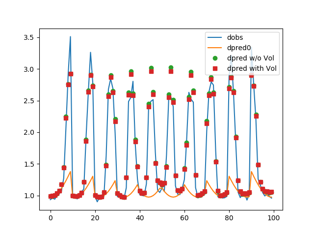
    # plot results

    if plotIt:

        fig, ax = plt.subplots(1, 1)
        ax.plot(data.dobs)
        ax.plot(dpred)
        ax.plot(problem.dpred(mopt1), "o")
        ax.plot(problem.dpred(mopt2), "s")
        ax.legend(["dobs", "dpred0", "dpred w/o Vol", "dpred with Vol"])

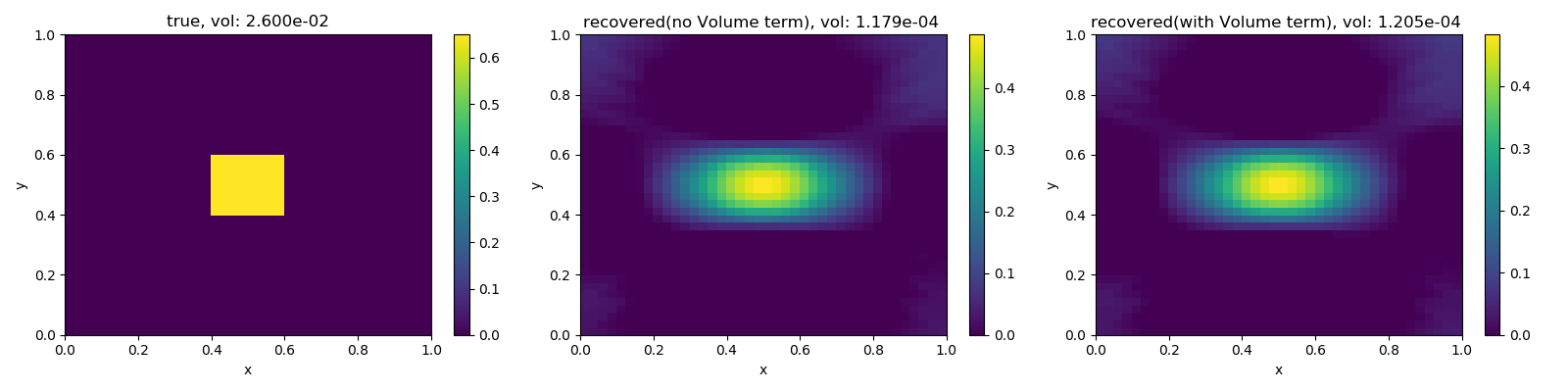
        fig, ax = plt.subplots(1, 3, figsize=(16, 4))
        cb0 = plt.colorbar(M.plotImage(phitrue, ax=ax[0])[0], ax=ax[0])
        cb1 = plt.colorbar(M.plotImage(mopt1, ax=ax[1])[0], ax=ax[1])
        cb2 = plt.colorbar(M.plotImage(mopt2, ax=ax[2])[0], ax=ax[2])

        for cb in [cb0, cb1, cb2]:
            cb.set_clim([0.0, phi1])

        ax[0].set_title("true, vol: {:1.3e}".format(knownVolume))
        ax[1].set_title(
            "recovered(no Volume term), vol: {:1.3e} ".format(dmisVol(mopt1))
        )
        ax[2].set_title(
            "recovered(with Volume term), vol: {:1.3e} ".format(dmisVol(mopt2))
        )

        plt.tight_layout()


if __name__ == "__main__":
    run()
    plt.show()