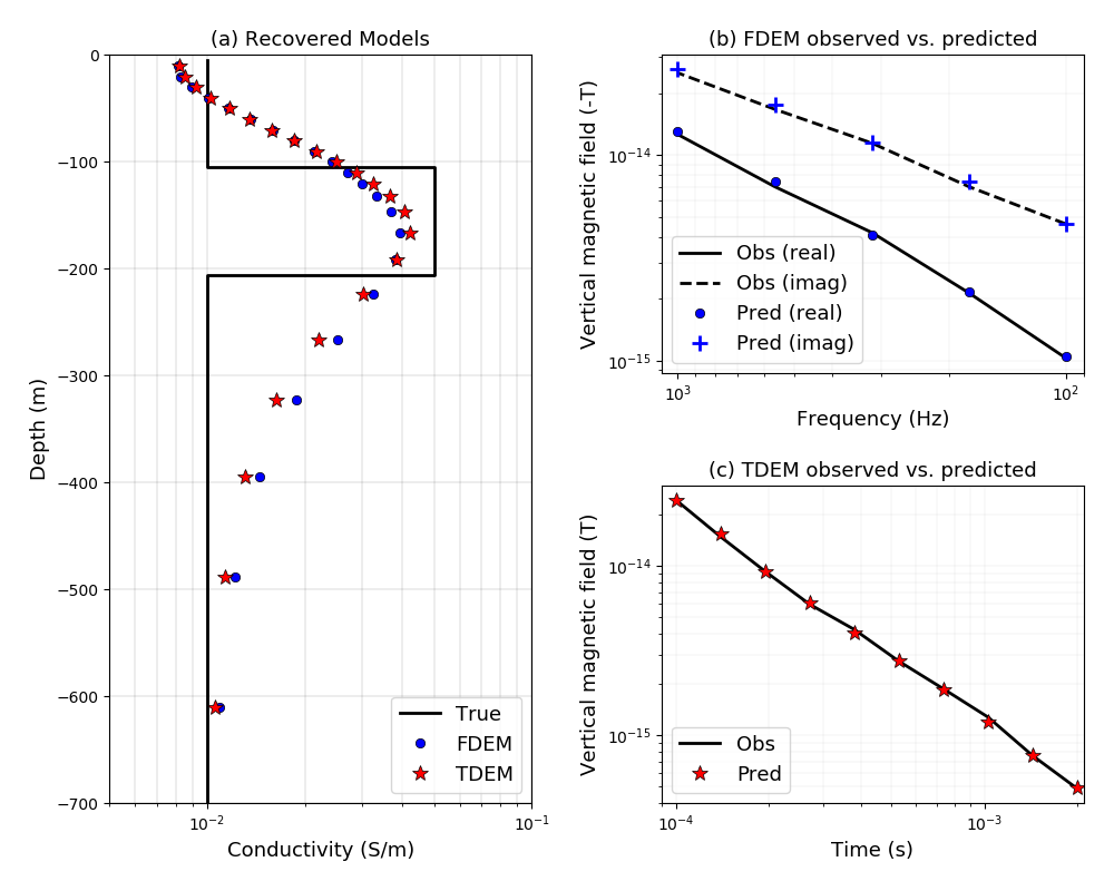
Heagy et al., 2017 1D FDEM and TDEM inversions

Here, we perform a 1D inversion using both the frequency and time domain codes. The forward simulations are conducted on a cylindrically symmetric mesh. The source is a point magnetic dipole source.

This example is used in the paper

Lindsey J. Heagy, Rowan Cockett, Seogi Kang, Gudni K. Rosenkjaer, Douglas W. Oldenburg, A framework for simulation and inversion in electromagnetics, Computers & Geosciences, Volume 107, 2017, Pages 1-19, ISSN 0098-3004, http://dx.doi.org/10.1016/j.cageo.2017.06.018.

This example is on figshare: https://doi.org/10.6084/m9.figshare.5035175

This example was updated for SimPEG 0.14.0 on January 31st, 2020 by Joseph Capriotti

Out:

min skin depth =  158.11388300841895 max skin depth =  500.0
max x  1267.687908603637 min z  -1242.6879086036365 max z  1242.687908603637
SimPEG.InvProblem will set Regularization.mref to m0.

        SimPEG.InvProblem is setting bfgsH0 to the inverse of the eval2Deriv.
        ***Done using same Solver and solverOpts as the problem***
model has any nan: 0
============================ Inexact Gauss Newton ============================
  #     beta     phi_d     phi_m       f      |proj(x-g)-x|  LS    Comment
-----------------------------------------------------------------------------
x0 has any nan: 0
   0  1.24e+02  7.81e+02  0.00e+00  7.81e+02    5.64e+02      0
   1  1.24e+02  2.61e+02  8.52e-01  3.66e+02    5.57e+01      0
   2  1.24e+02  2.07e+02  1.20e+00  3.55e+02    1.60e+01      0   Skip BFGS
   3  3.10e+01  1.95e+02  1.29e+00  2.35e+02    1.24e+02      0   Skip BFGS
   4  3.10e+01  2.76e+01  3.66e+00  1.41e+02    4.15e+01      0
   5  3.10e+01  2.39e+01  3.69e+00  1.38e+02    3.40e+00      0
   6  7.74e+00  2.32e+01  3.71e+00  5.20e+01    5.44e+01      0   Skip BFGS
------------------------- STOP! -------------------------
1 : |fc-fOld| = 0.0000e+00 <= tolF*(1+|f0|) = 7.8164e+01
1 : |xc-x_last| = 4.1565e-01 <= tolX*(1+|x0|) = 2.4026e+00
0 : |proj(x-g)-x|    = 5.4389e+01 <= tolG          = 1.0000e-01
0 : |proj(x-g)-x|    = 5.4389e+01 <= 1e3*eps       = 1.0000e-02
0 : maxIter   =      20    <= iter          =      7
------------------------- DONE! -------------------------
min diffusion distance  114.18394343377736 max diffusion distance  510.64611891383385
SimPEG.InvProblem will set Regularization.mref to m0.

        SimPEG.InvProblem is setting bfgsH0 to the inverse of the eval2Deriv.
        ***Done using same Solver and solverOpts as the problem***
model has any nan: 0
============================ Inexact Gauss Newton ============================
  #     beta     phi_d     phi_m       f      |proj(x-g)-x|  LS    Comment
-----------------------------------------------------------------------------
x0 has any nan: 0
   0  1.04e+02  1.64e+03  0.00e+00  1.64e+03    7.18e+02      0
   1  1.04e+02  1.48e+02  2.94e+00  4.55e+02    1.43e+02      0
   2  1.04e+02  9.85e+01  3.13e+00  4.25e+02    2.11e+01      0
   3  2.61e+01  9.37e+01  3.16e+00  1.76e+02    1.65e+02      0   Skip BFGS
   4  2.61e+01  1.27e+01  4.46e+00  1.29e+02    1.38e+01      0
   5  2.61e+01  1.25e+01  4.44e+00  1.28e+02    2.01e+00      0
   6  6.52e+00  1.23e+01  4.44e+00  4.13e+01    5.03e+01      0   Skip BFGS
------------------------- STOP! -------------------------
1 : |fc-fOld| = 0.0000e+00 <= tolF*(1+|f0|) = 1.6404e+02
1 : |xc-x_last| = 3.5884e-01 <= tolX*(1+|x0|) = 2.4026e+00
0 : |proj(x-g)-x|    = 5.0267e+01 <= tolG          = 1.0000e-01
0 : |proj(x-g)-x|    = 5.0267e+01 <= 1e3*eps       = 1.0000e-02
0 : maxIter   =      20    <= iter          =      7
------------------------- DONE! -------------------------
/Users/josephcapriotti/codes/simpeg/examples/20-published/plot_heagyetal2017_cyl_inversions.py:274: UserWarning: Matplotlib is currently using agg, which is a non-GUI backend, so cannot show the figure.
  plt.show()

import discretize
from SimPEG import (
    maps,
    utils,
    data_misfit,
    regularization,
    optimization,
    inversion,
    inverse_problem,
    directives,
)
import numpy as np
from SimPEG.electromagnetics import frequency_domain as FDEM, time_domain as TDEM, mu_0
import matplotlib.pyplot as plt
import matplotlib

try:
    from pymatsolver import Pardiso as Solver
except ImportError:
    from SimPEG import SolverLU as Solver


def run(plotIt=True, saveFig=False):

    # Set up cylindrically symmeric mesh
    cs, ncx, ncz, npad = 10.0, 15, 25, 13  # padded cyl mesh
    hx = [(cs, ncx), (cs, npad, 1.3)]
    hz = [(cs, npad, -1.3), (cs, ncz), (cs, npad, 1.3)]
    mesh = discretize.CylMesh([hx, 1, hz], "00C")

    # Conductivity model
    layerz = np.r_[-200.0, -100.0]
    layer = (mesh.vectorCCz >= layerz[0]) & (mesh.vectorCCz <= layerz[1])
    active = mesh.vectorCCz < 0.0
    sig_half = 1e-2  # Half-space conductivity
    sig_air = 1e-8  # Air conductivity
    sig_layer = 5e-2  # Layer conductivity
    sigma = np.ones(mesh.nCz) * sig_air
    sigma[active] = sig_half
    sigma[layer] = sig_layer

    # Mapping
    actMap = maps.InjectActiveCells(mesh, active, np.log(1e-8), nC=mesh.nCz)
    mapping = maps.ExpMap(mesh) * maps.SurjectVertical1D(mesh) * actMap
    mtrue = np.log(sigma[active])

    # ----- FDEM problem & survey ----- #
    rxlocs = utils.ndgrid([np.r_[50.0], np.r_[0], np.r_[0.0]])
    bzr = FDEM.Rx.PointMagneticFluxDensitySecondary(rxlocs, "z", "real")
    bzi = FDEM.Rx.PointMagneticFluxDensitySecondary(rxlocs, "z", "imag")

    freqs = np.logspace(2, 3, 5)
    srcLoc = np.array([0.0, 0.0, 0.0])

    print(
        "min skin depth = ",
        500.0 / np.sqrt(freqs.max() * sig_half),
        "max skin depth = ",
        500.0 / np.sqrt(freqs.min() * sig_half),
    )
    print(
        "max x ",
        mesh.vectorCCx.max(),
        "min z ",
        mesh.vectorCCz.min(),
        "max z ",
        mesh.vectorCCz.max(),
    )

    srcList = [
        FDEM.Src.MagDipole([bzr, bzi], freq, srcLoc, orientation="Z") for freq in freqs
    ]

    surveyFD = FDEM.Survey(srcList)
    prbFD = FDEM.Simulation3DMagneticFluxDensity(
        mesh, survey=surveyFD, sigmaMap=mapping, solver=Solver
    )
    rel_err = 0.03
    dataFD = prbFD.make_synthetic_data(mtrue, relative_error=rel_err, add_noise=True)
    dataFD.noise_floor = np.linalg.norm(dataFD.dclean) * 1e-5

    # FDEM inversion
    np.random.seed(1)
    dmisfit = data_misfit.L2DataMisfit(simulation=prbFD, data=dataFD)
    regMesh = discretize.TensorMesh([mesh.hz[mapping.maps[-1].indActive]])
    reg = regularization.Simple(regMesh)
    opt = optimization.InexactGaussNewton(maxIterCG=10)
    invProb = inverse_problem.BaseInvProblem(dmisfit, reg, opt)

    # Inversion Directives
    beta = directives.BetaSchedule(coolingFactor=4, coolingRate=3)
    betaest = directives.BetaEstimate_ByEig(beta0_ratio=2.0)
    target = directives.TargetMisfit()
    directiveList = [beta, betaest, target]

    inv = inversion.BaseInversion(invProb, directiveList=directiveList)
    m0 = np.log(np.ones(mtrue.size) * sig_half)
    reg.alpha_s = 5e-1
    reg.alpha_x = 1.0
    prbFD.counter = opt.counter = utils.Counter()
    opt.remember("xc")
    moptFD = inv.run(m0)

    # TDEM problem
    times = np.logspace(-4, np.log10(2e-3), 10)
    print(
        "min diffusion distance ",
        1.28 * np.sqrt(times.min() / (sig_half * mu_0)),
        "max diffusion distance ",
        1.28 * np.sqrt(times.max() / (sig_half * mu_0)),
    )
    rx = TDEM.Rx.PointMagneticFluxDensity(rxlocs, times, "z")
    src = TDEM.Src.MagDipole(
        [rx],
        waveform=TDEM.Src.StepOffWaveform(),
        loc=srcLoc,  # same src location as FDEM problem
    )

    surveyTD = TDEM.Survey([src])
    prbTD = TDEM.Simulation3DMagneticFluxDensity(
        mesh, survey=surveyTD, sigmaMap=mapping, Solver=Solver
    )
    prbTD.time_steps = [(5e-5, 10), (1e-4, 10), (5e-4, 10)]

    rel_err = 0.03
    dataTD = prbTD.make_synthetic_data(mtrue, relative_error=rel_err, add_noise=True)
    dataTD.noise_floor = np.linalg.norm(dataTD.dclean) * 1e-5

    # TDEM inversion
    dmisfit = data_misfit.L2DataMisfit(simulation=prbTD, data=dataTD)
    regMesh = discretize.TensorMesh([mesh.hz[mapping.maps[-1].indActive]])
    reg = regularization.Simple(regMesh)
    opt = optimization.InexactGaussNewton(maxIterCG=10)
    invProb = inverse_problem.BaseInvProblem(dmisfit, reg, opt)

    # directives
    beta = directives.BetaSchedule(coolingFactor=4, coolingRate=3)
    betaest = directives.BetaEstimate_ByEig(beta0_ratio=2.0)
    target = directives.TargetMisfit()
    directiveList = [beta, betaest, target]

    inv = inversion.BaseInversion(invProb, directiveList=directiveList)
    m0 = np.log(np.ones(mtrue.size) * sig_half)
    reg.alpha_s = 5e-1
    reg.alpha_x = 1.0
    prbTD.counter = opt.counter = utils.Counter()
    opt.remember("xc")
    moptTD = inv.run(m0)

    # Plot the results
    if plotIt:
        plt.figure(figsize=(10, 8))
        ax0 = plt.subplot2grid((2, 2), (0, 0), rowspan=2)
        ax1 = plt.subplot2grid((2, 2), (0, 1))
        ax2 = plt.subplot2grid((2, 2), (1, 1))

        fs = 13  # fontsize
        matplotlib.rcParams["font.size"] = fs

        # Plot the model
        # z_true = np.repeat(mesh.vectorCCz[active][1:], 2, axis=0)
        # z_true = np.r_[mesh.vectorCCz[active][0], z_true, mesh.vectorCCz[active][-1]]
        activeN = mesh.vectorNz <= 0.0 + cs / 2.0
        z_true = np.repeat(mesh.vectorNz[activeN][1:-1], 2, axis=0)
        z_true = np.r_[mesh.vectorNz[activeN][0], z_true, mesh.vectorNz[activeN][-1]]
        sigma_true = np.repeat(sigma[active], 2, axis=0)

        ax0.semilogx(sigma_true, z_true, "k-", lw=2, label="True")

        ax0.semilogx(
            np.exp(moptFD),
            mesh.vectorCCz[active],
            "bo",
            ms=6,
            markeredgecolor="k",
            markeredgewidth=0.5,
            label="FDEM",
        )
        ax0.semilogx(
            np.exp(moptTD),
            mesh.vectorCCz[active],
            "r*",
            ms=10,
            markeredgecolor="k",
            markeredgewidth=0.5,
            label="TDEM",
        )
        ax0.set_ylim(-700, 0)
        ax0.set_xlim(5e-3, 1e-1)

        ax0.set_xlabel("Conductivity (S/m)", fontsize=fs)
        ax0.set_ylabel("Depth (m)", fontsize=fs)
        ax0.grid(which="both", color="k", alpha=0.5, linestyle="-", linewidth=0.2)
        ax0.legend(fontsize=fs, loc=4)

        # plot the data misfits - negative b/c we choose positive to be in the
        # direction of primary

        ax1.plot(freqs, -dataFD.dobs[::2], "k-", lw=2, label="Obs (real)")
        ax1.plot(freqs, -dataFD.dobs[1::2], "k--", lw=2, label="Obs (imag)")

        dpredFD = prbFD.dpred(moptTD)
        ax1.loglog(
            freqs,
            -dpredFD[::2],
            "bo",
            ms=6,
            markeredgecolor="k",
            markeredgewidth=0.5,
            label="Pred (real)",
        )
        ax1.loglog(
            freqs, -dpredFD[1::2], "b+", ms=10, markeredgewidth=2.0, label="Pred (imag)"
        )

        ax2.loglog(times, dataTD.dobs, "k-", lw=2, label="Obs")
        ax2.loglog(
            times,
            prbTD.dpred(moptTD),
            "r*",
            ms=10,
            markeredgecolor="k",
            markeredgewidth=0.5,
            label="Pred",
        )
        ax2.set_xlim(times.min() - 1e-5, times.max() + 1e-4)

        # Labels, gridlines, etc
        ax2.grid(which="both", alpha=0.5, linestyle="-", linewidth=0.2)
        ax1.grid(which="both", alpha=0.5, linestyle="-", linewidth=0.2)

        ax1.set_xlabel("Frequency (Hz)", fontsize=fs)
        ax1.set_ylabel("Vertical magnetic field (-T)", fontsize=fs)

        ax2.set_xlabel("Time (s)", fontsize=fs)
        ax2.set_ylabel("Vertical magnetic field (T)", fontsize=fs)

        ax2.legend(fontsize=fs, loc=3)
        ax1.legend(fontsize=fs, loc=3)
        ax1.set_xlim(freqs.max() + 1e2, freqs.min() - 1e1)

        ax0.set_title("(a) Recovered Models", fontsize=fs)
        ax1.set_title("(b) FDEM observed vs. predicted", fontsize=fs)
        ax2.set_title("(c) TDEM observed vs. predicted", fontsize=fs)

        plt.tight_layout(pad=1.5)

        if saveFig is True:
            plt.savefig("example1.png", dpi=600)


if __name__ == "__main__":
    run(plotIt=True, saveFig=True)
    plt.show()