Simulate a 1D Sounding over a Layered Earth

Here we use the module SimPEG.electromangetics.static.resistivity to predict sounding data over a 1D layered Earth. In this tutorial, we focus on the following:

• General definition of sources and receivers

• How to define the survey

• How to predict voltage or apparent resistivity data

• The units of the model and resulting data

• 1D simulation for DC resistivity

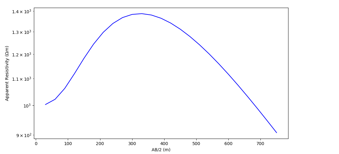
For this tutorial, we will simulate sounding data over a layered Earth using a Wenner array. The end product is a sounding curve which tells us how the electrical resistivity changes with depth.

Import modules

import os
import numpy as np
import matplotlib.pyplot as plt

from discretize import TensorMesh

from SimPEG import maps
from SimPEG.electromagnetics.static import resistivity as dc
from SimPEG.electromagnetics.static.utils.static_utils import plot_layer

save_file = False

# sphinx_gallery_thumbnail_number = 2

Create Survey

Here we demonstrate a general way to define sources and receivers. For pole and dipole sources, we must define the A or AB electrode locations, respectively. For the pole and dipole receivers, we must define the M or MN electrode locations, respectively.

a_min = 20.0
a_max = 500.0
n_stations = 25

# Define the 'a' spacing for Wenner array measurements for each reading
electrode_separations = np.linspace(a_min, a_max, n_stations)

source_list = []  # create empty array for sources to live

for ii in range(0, len(electrode_separations)):

    # Extract separation parameter for sources and receivers
    a = electrode_separations[ii]

    # AB electrode locations for source. Each is a (1, 3) numpy array
    A_location = np.r_[-1.5 * a, 0.0, 0.0]
    B_location = np.r_[1.5 * a, 0.0, 0.0]

    # MN electrode locations for receivers. Each is an (N, 3) numpy array
    M_location = np.r_[-0.5 * a, 0.0, 0.0]
    N_location = np.r_[0.5 * a, 0.0, 0.0]

    # Create receivers list. Define as pole or dipole.
    receiver_list = dc.receivers.Dipole(M_location, N_location)
    receiver_list = [receiver_list]

    # Define the source properties and associated receivers
    source_list.append(dc.sources.Dipole(receiver_list, A_location, B_location))

# Define survey
survey = dc.Survey(source_list)

Defining a 1D Layered Earth Model

Here, we define the layer thicknesses and electrical resistivities for our 1D simulation. If we have N layers, we define N electrical resistivity values and N-1 layer thicknesses. The lowest layer is assumed to extend to infinity.

# Define layer thicknesses.
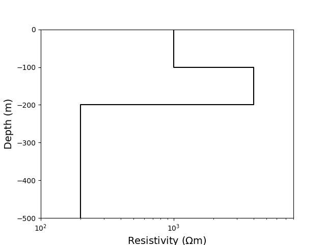
layer_thicknesses = np.r_[100.0, 100.0]

# Define layer resistivities.
model = np.r_[1e3, 4e3, 2e2]

# Define mapping from model to 1D layers.
model_map = maps.IdentityMap(nP=len(model))

Plot Resistivity Model

Here we plot the 1D resistivity model.

# Define a 1D mesh for plotting. Provide a maximum depth for the plot.
max_depth = 500
mesh = TensorMesh([np.r_[layer_thicknesses, max_depth - layer_thicknesses.sum()]])

# Plot the 1D model
plot_layer(model_map * model, mesh)

Out:

[<matplotlib.lines.Line2D object at 0x1823ba7048>]

Define the Forward Simulation and Predict DC Resistivity Data

Here we predict DC resistivity data. If the keyword argument rhoMap is defined, the simulation will expect a resistivity model. If the keyword argument sigmaMap is defined, the simulation will expect a conductivity model.

simulation = dc.simulation_1d.Simulation1DLayers(
    survey=survey,
    rhoMap=model_map,
    thicknesses=layer_thicknesses,
    data_type="apparent_resistivity",
)

# Predict data for a given model
dpred = simulation.dpred(model)

# Plot apparent resistivities on sounding curve
fig = plt.figure(figsize=(11, 5))
ax1 = fig.add_axes([0.1, 0.1, 0.75, 0.85])
ax1.semilogy(1.5 * electrode_separations, dpred, "b")
ax1.set_xlabel("AB/2 (m)")
ax1.set_ylabel("Apparent Resistivity ($\Omega m$)")
plt.show()

Out:

* ERROR   :: <ht> must be one of: ['dlf', 'qwe', 'quad']; <ht> provided: fht
/Users/josephcapriotti/codes/simpeg/tutorials/05-dcr/plot_fwd_1_dcr_sounding.py:143: UserWarning: Matplotlib is currently using agg, which is a non-GUI backend, so cannot show the figure.
  plt.show()

Optional: Export Data

Export data and true model

if save_file:

    dir_path = os.path.dirname(dc.__file__).split(os.path.sep)[:-4]
    dir_path.extend(["tutorials", "assets", "dcr1d"])
    dir_path = os.path.sep.join(dir_path) + os.path.sep

    noise = 0.025 * dpred * np.random.rand(len(dpred))

    data_array = np.c_[
        survey.locations_a,
        survey.locations_b,
        survey.locations_m,
        survey.locations_n,
        dpred + noise,
    ]

    fname = dir_path + "app_res_1d_data.dobs"
    np.savetxt(fname, data_array, fmt="%.4e")

    fname = dir_path + "true_model.txt"
    np.savetxt(fname, model, fmt="%.4e")

    fname = dir_path + "layers.txt"
    np.savetxt(fname, mesh.hx, fmt="%d")