Parametric 1D Inversion of Sounding Data¶

Here we use the module SimPEG.electromangetics.static.resistivity to invert DC resistivity sounding data and recover the resistivities and layer thicknesses for a 1D layered Earth. In this tutorial, we focus on the following:

How to define sources and receivers from a survey file

How to define the survey

Defining a model that consists of resistivities and layer thicknesses

For this tutorial, we will invert sounding data collected over a layered Earth using a Wenner array. The end product is layered Earth model which explains the data.

Import modules¶

import os
import numpy as np
import matplotlib as mpl
import matplotlib.pyplot as plt
import tarfile

from discretize import TensorMesh

from SimPEG import (
    maps,
    data,
    data_misfit,
    regularization,
    optimization,
    inverse_problem,
    inversion,
    directives,
    utils,
)
from SimPEG.electromagnetics.static import resistivity as dc
from SimPEG.electromagnetics.static.utils.static_utils import plot_layer

# sphinx_gallery_thumbnail_number = 2

Define File Names¶

Here we provide the file paths to assets we need to run the inversion. The Path to the true model is also provided for comparison with the inversion results. These files are stored as a tar-file on our google cloud bucket: “https://storage.googleapis.com/simpeg/doc-assets/dcip1d.tar.gz”

# storage bucket where we have the data
data_source = "https://storage.googleapis.com/simpeg/doc-assets/dcip1d.tar.gz"

# download the data
downloaded_data = utils.download(data_source, overwrite=True)

# unzip the tarfile
tar = tarfile.open(downloaded_data, "r")
tar.extractall()
tar.close()

# path to the directory containing our data
dir_path = downloaded_data.split(".")[0] + os.path.sep

# files to work with
data_filename = dir_path + "app_res_1d_data.dobs"
model_filename = dir_path + "true_model.txt"
mesh_filename = dir_path + "layers.txt"

Out:

overwriting /Users/josephcapriotti/codes/simpeg/tutorials/05-dcr/dcip1d.tar.gz
Downloading https://storage.googleapis.com/simpeg/doc-assets/dcip1d.tar.gz
   saved to: /Users/josephcapriotti/codes/simpeg/tutorials/05-dcr/dcip1d.tar.gz
Download completed!

Load Data, Define Survey and Plot¶

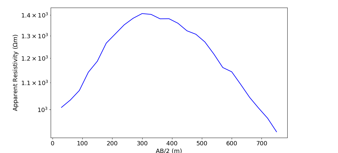
Here we load the observed data, define the DC survey geometry and plot the data values.

# Load data
dobs = np.loadtxt(str(data_filename))

A_electrodes = dobs[:, 0:3]
B_electrodes = dobs[:, 3:6]
M_electrodes = dobs[:, 6:9]
N_electrodes = dobs[:, 9:12]
dobs = dobs[:, -1]

# Define survey
unique_tx, k = np.unique(np.c_[A_electrodes, B_electrodes], axis=0, return_index=True)
n_sources = len(k)
k = np.sort(k)
k = np.r_[k, len(k) + 1]

source_list = []
for ii in range(0, n_sources):

    # MN electrode locations for receivers. Each is an (N, 3) numpy array
    M_locations = M_electrodes[k[ii] : k[ii + 1], :]
    N_locations = N_electrodes[k[ii] : k[ii + 1], :]
    receiver_list = [dc.receivers.Dipole(M_locations, N_locations)]

    # AB electrode locations for source. Each is a (1, 3) numpy array
    A_location = A_electrodes[k[ii], :]
    B_location = B_electrodes[k[ii], :]
    source_list.append(dc.sources.Dipole(receiver_list, A_location, B_location))

# Define survey
survey = dc.Survey(source_list)

# Plot apparent resistivities on sounding curve as a function of Wenner separation
# parameter.
electrode_separations = 0.5 * np.sqrt(
    np.sum((survey.locations_a - survey.locations_b) ** 2, axis=1)
)

fig = plt.figure(figsize=(11, 5))
mpl.rcParams.update({"font.size": 14})
ax1 = fig.add_axes([0.15, 0.1, 0.7, 0.85])
ax1.semilogy(electrode_separations, dobs, "b")
ax1.set_xlabel("AB/2 (m)")
ax1.set_ylabel("Apparent Resistivity ($\Omega m$)")
plt.show()

Out:

/Users/josephcapriotti/codes/simpeg/tutorials/05-dcr/plot_inv_1_dcr_sounding_parametric.py:132: UserWarning: Matplotlib is currently using agg, which is a non-GUI backend, so cannot show the figure.
  plt.show()

Assign Uncertainties¶

Inversion with SimPEG requires that we define standard deviation on our data. This represents our estimate of the noise in our data. For DC sounding data, a relative error is applied to each datum. For this tutorial, the relative error on each datum will be 2.5%.

std = 0.025 * dobs

Define Data¶

Here is where we define the data that are inverted. The data are defined by the survey, the observation values and the standard deviation.

data_object = data.Data(survey, dobs=dobs, standard_deviation=std)

Defining the Starting Model and Mapping¶

In this case, the model consists of parameters which define the respective resistivities and thickness for a set of horizontal layer. Here, we choose to define a model consisting of 3 layers.

# Define the resistivities and thicknesses for the starting model. The thickness
# of the bottom layer is assumed to extend downward to infinity so we don't
# need to define it.
resistivities = np.r_[1e3, 1e3, 1e3]
layer_thicknesses = np.r_[50.0, 50.0]

# Define a mesh for plotting and regularization.
mesh = TensorMesh([(np.r_[layer_thicknesses, layer_thicknesses[-1]])], "0")
print(mesh)

# Define model. We are inverting for the layer resistivities and layer thicknesses.
# Since the bottom layer extends to infinity, it is not a model parameter for
# which we need to invert. For a 3 layer model, there is a total of 5 parameters.
# For stability, our model is the log-resistivity and log-thickness.
starting_model = np.r_[np.log(resistivities), np.log(layer_thicknesses)]

# Since the model contains two different properties for each layer, we use
# wire maps to distinguish the properties.
wire_map = maps.Wires(("rho", mesh.nC), ("t", mesh.nC - 1))
resistivity_map = maps.ExpMap(nP=mesh.nC) * wire_map.rho
layer_map = maps.ExpMap(nP=mesh.nC - 1) * wire_map.t

Out:

TensorMesh: 3 cells

                    MESH EXTENT             CELL WIDTH      FACTOR
dir    nC        min           max         min       max      max
---   ---  ---------------------------  ------------------  ------
 x      3          0.00        150.00     50.00     50.00    1.00

Define the Physics¶

Here we define the physics of the problem. The data consists of apparent resistivity values. This is defined here.

simulation = dc.simulation_1d.Simulation1DLayers(
    survey=survey,
    rhoMap=resistivity_map,
    thicknessesMap=layer_map,
    data_type="apparent_resistivity",
)

Out:

* ERROR   :: <ht> must be one of: ['dlf', 'qwe', 'quad']; <ht> provided: fht

Define Inverse Problem¶

The inverse problem is defined by 3 things:

Data Misfit: a measure of how well our recovered model explains the field data

Regularization: constraints placed on the recovered model and a priori information

Optimization: the numerical approach used to solve the inverse problem

# Define the data misfit. Here the data misfit is the L2 norm of the weighted
# residual between the observed data and the data predicted for a given model.
# Within the data misfit, the residual between predicted and observed data are
# normalized by the data's standard deviation.
dmis = data_misfit.L2DataMisfit(simulation=simulation, data=data_object)

# Define the regularization on the parameters related to resistivity
mesh_rho = TensorMesh([mesh.hx.size])
reg_rho = regularization.Simple(mesh_rho, alpha_s=0.01, alpha_x=1, mapping=wire_map.rho)

# Define the regularization on the parameters related to layer thickness
mesh_t = TensorMesh([mesh.hx.size - 1])
reg_t = regularization.Simple(mesh_t, alpha_s=0.01, alpha_x=1, mapping=wire_map.t)

# Combine to make regularization for the inversion problem
reg = reg_rho + reg_t

# Define how the optimization problem is solved. Here we will use an inexact
# Gauss-Newton approach that employs the conjugate gradient solver.
opt = optimization.InexactGaussNewton(maxIter=50, maxIterCG=30)

# Define the inverse problem
inv_prob = inverse_problem.BaseInvProblem(dmis, reg, opt)

Define Inversion Directives¶

Here we define any directives that are carried out during the inversion. This includes the cooling schedule for the trade-off parameter (beta), stopping criteria for the inversion and saving inversion results at each iteration.

# Apply and update sensitivity weighting as the model updates
update_sensitivity_weights = directives.UpdateSensitivityWeights()

# Defining a starting value for the trade-off parameter (beta) between the data
# misfit and the regularization.
starting_beta = directives.BetaEstimate_ByEig(beta0_ratio=1e1)

# Set the rate of reduction in trade-off parameter (beta) each time the
# the inverse problem is solved. And set the number of Gauss-Newton iterations
# for each trade-off paramter value.
beta_schedule = directives.BetaSchedule(coolingFactor=5.0, coolingRate=3.0)

# Options for outputting recovered models and predicted data for each beta.
save_iteration = directives.SaveOutputEveryIteration(save_txt=False)

# Setting a stopping criteria for the inversion.
target_misfit = directives.TargetMisfit(chifact=0.1)

# The directives are defined in a list
directives_list = [
    update_sensitivity_weights,
    starting_beta,
    beta_schedule,
    target_misfit,
]

Running the Inversion¶

To define the inversion object, we need to define the inversion problem and the set of directives. We can then run the inversion.

# Here we combine the inverse problem and the set of directives
inv = inversion.BaseInversion(inv_prob, directiveList=directives_list)

# Run the inversion
recovered_model = inv.run(starting_model)

Out:

SimPEG.InvProblem will set Regularization.mref to m0.
SimPEG.InvProblem will set Regularization.mref to m0.

        SimPEG.InvProblem is setting bfgsH0 to the inverse of the eval2Deriv.
        ***Done using same Solver and solverOpts as the problem***
model has any nan: 0
============================ Inexact Gauss Newton ============================
  #     beta     phi_d     phi_m       f      |proj(x-g)-x|  LS    Comment
-----------------------------------------------------------------------------
x0 has any nan: 0
5.83e+04  7.44e+02  0.00e+00  7.44e+02    3.04e+03      0
5.83e+04  3.40e+02  2.67e-04  3.56e+02    2.88e+02      0
5.83e+04  3.39e+02  2.43e-04  3.53e+02    1.60e+01      0
1.17e+04  3.39e+02  2.10e-04  3.41e+02    4.11e+02      1
1.17e+04  3.27e+02  7.05e-04  3.35e+02    4.29e+01      0
1.17e+04  3.25e+02  6.21e-04  3.33e+02    2.03e+02      2
2.33e+03  3.25e+02  6.66e-04  3.27e+02    2.35e+02      2
2.33e+03  3.22e+02  9.28e-04  3.24e+02    2.69e+02      2
2.33e+03  3.19e+02  1.18e-03  3.22e+02    1.51e+02      2
4.66e+02  3.16e+02  1.75e-03  3.17e+02    1.66e+02      1
4.66e+02  3.06e+02  9.48e-03  3.11e+02    1.77e+02      0
4.66e+02  2.71e+02  3.95e-02  2.89e+02    9.13e+02      1
9.32e+01  2.33e+02  1.37e-01  2.46e+02    1.06e+03      1
9.32e+01  1.55e+02  7.55e-01  2.26e+02    2.09e+03      0   Skip BFGS
9.32e+01  4.34e+01  7.43e-01  1.13e+02    6.03e+01      0
1.86e+01  3.85e+01  7.66e-01  5.28e+01    1.50e+02      0
1.86e+01  2.53e+01  1.03e+00  4.44e+01    3.88e+02      1
1.86e+01  1.02e+01  1.37e+00  3.56e+01    1.89e+02      0   Skip BFGS
3.73e+00  9.40e+00  1.31e+00  1.43e+01    1.28e+02      1
3.73e+00  5.28e+00  1.58e+00  1.12e+01    1.24e+02      1
3.73e+00  3.58e+00  1.79e+00  1.02e+01    5.96e+01      1   Skip BFGS
7.46e-01  2.90e+00  1.82e+00  4.25e+00    6.51e+01      1
7.46e-01  1.45e+00  2.42e+00  3.26e+00    9.93e+01      0
------------------------- STOP! -------------------------
: |fc-fOld| = 0.0000e+00 <= tolF*(1+|f0|) = 7.4460e+01
: |xc-x_last| = 5.9834e-02 <= tolX*(1+|x0|) = 1.4182e+00
: |proj(x-g)-x|    = 9.9313e+01 <= tolG          = 1.0000e-01
: |proj(x-g)-x|    = 9.9313e+01 <= 1e3*eps       = 1.0000e-02
: maxIter   =      50    <= iter          =     23
------------------------- DONE! -------------------------

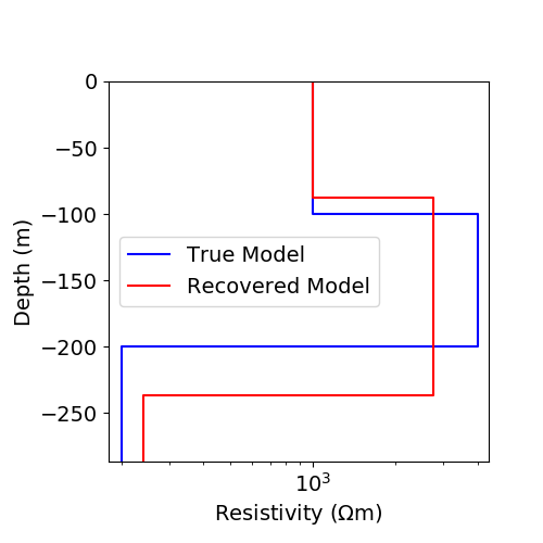
Examining the Results¶

# Load the true model and layer thicknesses
true_model = np.loadtxt(str(model_filename))
true_layers = np.loadtxt(str(mesh_filename))
true_layers = TensorMesh([true_layers], "0")

# Plot true model and recovered model
fig = plt.figure(figsize=(5, 5))
plotting_mesh = TensorMesh(
    [np.r_[layer_map * recovered_model, layer_thicknesses[-1]]], "0"
)
x_min = np.min([np.min(resistivity_map * recovered_model), np.min(true_model)])
x_max = np.max([np.max(resistivity_map * recovered_model), np.max(true_model)])

ax1 = fig.add_axes([0.2, 0.15, 0.7, 0.7])
plot_layer(true_model, true_layers, ax=ax1, depth_axis=False, color="b")
plot_layer(
    resistivity_map * recovered_model,
    plotting_mesh,
    ax=ax1,
    depth_axis=False,
    color="r",
)
ax1.set_xlim(0.9 * x_min, 1.1 * x_max)
ax1.legend(["True Model", "Recovered Model"])

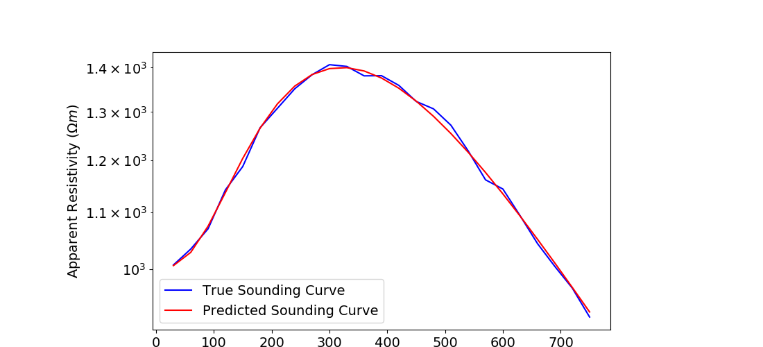
# Plot the true and apparent resistivities on a sounding curve
fig = plt.figure(figsize=(11, 5))
ax1 = fig.add_axes([0.2, 0.05, 0.6, 0.8])
ax1.semilogy(electrode_separations, dobs, "b")
ax1.semilogy(electrode_separations, inv_prob.dpred, "r")
ax1.set_xlabel("AB/2 (m)")
ax1.set_ylabel("Apparent Resistivity ($\Omega m$)")
ax1.legend(["True Sounding Curve", "Predicted Sounding Curve"])
plt.show()

Out:

/Users/josephcapriotti/codes/simpeg/tutorials/05-dcr/plot_inv_1_dcr_sounding_parametric.py:326: UserWarning: Matplotlib is currently using agg, which is a non-GUI backend, so cannot show the figure.
  plt.show()

Total running time of the script: ( 0 minutes 7.255 seconds)

Download Python source code: plot_inv_1_dcr_sounding_parametric.py

Download Jupyter notebook: plot_inv_1_dcr_sounding_parametric.ipynb

Gallery generated by Sphinx-Gallery