2.5D DC Resistivity Least-Squares Inversion

Here we invert a line of DC resistivity data to recover an electrical conductivity model. We formulate the inverse problem as a least-squares optimization problem. For this tutorial, we focus on the following:

• Defining the survey

• Generating a mesh based on survey geometry

• Including surface topography

• Defining the inverse problem (data misfit, regularization, directives)

• Applying sensitivity weighting

• Plotting the recovered model and data misfit

Import modules

import os
import numpy as np
import matplotlib as mpl
import matplotlib.pyplot as plt
import tarfile

from discretize import TreeMesh
from discretize.utils import mkvc, refine_tree_xyz

from SimPEG.utils import surface2ind_topo
from SimPEG import (
    maps,
    data,
    data_misfit,
    regularization,
    optimization,
    inverse_problem,
    inversion,
    directives,
    utils,
)
from SimPEG.electromagnetics.static import resistivity as dc
from SimPEG.electromagnetics.static.utils.static_utils import plot_pseudoSection

try:
    from pymatsolver import Pardiso as Solver
except ImportError:
    from SimPEG import SolverLU as Solver

# sphinx_gallery_thumbnail_number = 2

Define File Names

Here we provide the file paths to assets we need to run the inversion. The path to the true model conductivity and chargeability models are also provided for comparison with the inversion results. These files are stored as a tar-file on our google cloud bucket: “https://storage.googleapis.com/simpeg/doc-assets/dcip2d.tar.gz”

# storage bucket where we have the data
data_source = "https://storage.googleapis.com/simpeg/doc-assets/dcip2d.tar.gz"

# download the data
downloaded_data = utils.download(data_source, overwrite=True)

# unzip the tarfile
tar = tarfile.open(downloaded_data, "r")
tar.extractall()
tar.close()

# path to the directory containing our data
dir_path = downloaded_data.split(".")[0] + os.path.sep

# files to work with
topo_filename = dir_path + "xyz_topo.txt"
data_filename = dir_path + "dc_data.obs"
true_conductivity_filename = dir_path + "true_conductivity.txt"

Out:

overwriting /Users/josephcapriotti/codes/simpeg/tutorials/05-dcr/dcip2d.tar.gz
Downloading https://storage.googleapis.com/simpeg/doc-assets/dcip2d.tar.gz
   saved to: /Users/josephcapriotti/codes/simpeg/tutorials/05-dcr/dcip2d.tar.gz
Download completed!

Load Data, Define Survey and Plot

Here we load the observed data, define the DC and IP survey geometry and plot the data values using pseudo-sections.

# Load data
topo_xyz = np.loadtxt(str(topo_filename))
dobs = np.loadtxt(str(data_filename))

# Extract source and receiver electrode locations and the observed data
A_electrodes = dobs[:, 0:2]
B_electrodes = dobs[:, 2:4]
M_electrodes = dobs[:, 4:6]
N_electrodes = dobs[:, 6:8]
dobs = dobs[:, -1]

# Define survey
unique_tx, k = np.unique(np.c_[A_electrodes, B_electrodes], axis=0, return_index=True)
n_sources = len(k)
k = np.r_[k, len(A_electrodes) + 1]

source_list = []
for ii in range(0, n_sources):

    # MN electrode locations for receivers. Each is an (N, 3) numpy array
    M_locations = M_electrodes[k[ii] : k[ii + 1], :]
    N_locations = N_electrodes[k[ii] : k[ii + 1], :]
    receiver_list = [dc.receivers.Dipole(M_locations, N_locations, data_type="volt")]

    # AB electrode locations for source. Each is a (1, 3) numpy array
    A_location = A_electrodes[k[ii], :]
    B_location = B_electrodes[k[ii], :]
    source_list.append(dc.sources.Dipole(receiver_list, A_location, B_location))

# Define survey
survey = dc.survey.Survey_ky(source_list)

# Define the a data object. Uncertainties are added later
dc_data = data.Data(survey, dobs=dobs)

# Plot apparent conductivity using pseudo-section
mpl.rcParams.update({"font.size": 12})
fig = plt.figure(figsize=(12, 5))

ax1 = fig.add_axes([0.05, 0.05, 0.8, 0.9])
plot_pseudoSection(
    dc_data,
    ax=ax1,
    survey_type="dipole-dipole",
    data_type="appConductivity",
    space_type="half-space",
    scale="log",
    pcolorOpts={"cmap": "viridis"},
)
ax1.set_title("Apparent Conductivity [S/m]")

plt.show()

Out:

/Users/josephcapriotti/codes/simpeg/tutorials/05-dcr/plot_inv_2_dcr2d.py:146: UserWarning: Matplotlib is currently using agg, which is a non-GUI backend, so cannot show the figure.
  plt.show()

Assign Uncertainties

Inversion with SimPEG requires that we define standard deviation on our data. This represents our estimate of the noise in our data. For DC data, a relative error is applied to each datum.

# Compute standard deviations
std = 0.05 * np.abs(dobs)

# Add standard deviations to data object
dc_data.standard_deviation = std

Create OcTree Mesh

Here, we create the OcTree mesh that will be used to predict both DC resistivity and IP data.

dh = 10.0  # base cell width
dom_width_x = 2400.0  # domain width x
dom_width_z = 1200.0  # domain width z
nbcx = 2 ** int(np.round(np.log(dom_width_x / dh) / np.log(2.0)))  # num. base cells x
nbcz = 2 ** int(np.round(np.log(dom_width_z / dh) / np.log(2.0)))  # num. base cells z

# Define the base mesh
hx = [(dh, nbcx)]
hz = [(dh, nbcz)]
mesh = TreeMesh([hx, hz], x0="CN")

# Mesh refinement based on topography
mesh = refine_tree_xyz(
    mesh, topo_xyz[:, [0, 2]], octree_levels=[1], method="surface", finalize=False
)

# Mesh refinement near transmitters and receivers
electrode_locations = np.r_[
    survey.locations_a, survey.locations_b, survey.locations_m, survey.locations_n
]

unique_locations = np.unique(electrode_locations, axis=0)

mesh = refine_tree_xyz(
    mesh, unique_locations, octree_levels=[2, 4], method="radial", finalize=False
)

# Refine core mesh region
xp, zp = np.meshgrid([-800.0, 800.0], [-800.0, 0.0])
xyz = np.c_[mkvc(xp), mkvc(zp)]
mesh = refine_tree_xyz(mesh, xyz, octree_levels=[0, 2, 2], method="box", finalize=False)

mesh.finalize()

Project Surveys to Discretized Topography

It is important that electrodes are not model as being in the air. Even if the electrodes are properly located along surface topography, they may lie above the discretized topography. This step is carried out to ensure all electrodes like on the discretized surface.

# Find cells that lie below surface topography
ind_active = surface2ind_topo(mesh, topo_xyz[:, [0, 2]])

# Shift electrodes to the surface of discretized topography
survey.drape_electrodes_on_topography(mesh, ind_active, option="top")

Starting/Reference Model and Mapping on OcTree Mesh

Here, we would create starting and/or reference models for the DC inversion as well as the mapping from the model space to the active cells. Starting and reference models can be a constant background value or contain a-priori structures. Here, the starting model is the natural log of 0.01 S/m.

# Define conductivity model in S/m (or resistivity model in Ohm m)
air_conductivity = np.log(1e-8)
background_conductivity = np.log(1e-2)

active_map = maps.InjectActiveCells(mesh, ind_active, np.exp(air_conductivity))
nC = int(ind_active.sum())

conductivity_map = active_map * maps.ExpMap()

# Define model
starting_conductivity_model = background_conductivity * np.ones(nC)

Define the Physics of the DC Simulation

Here, we define the physics of the DC resistivity problem.

# Define the problem. Define the cells below topography and the mapping
simulation = dc.simulation_2d.Simulation2DNodal(
    mesh, survey=survey, sigmaMap=conductivity_map, Solver=Solver
)

Define DC Inverse Problem

The inverse problem is defined by 3 things:

1. Data Misfit: a measure of how well our recovered model explains the field data

2. Regularization: constraints placed on the recovered model and a priori information

3. Optimization: the numerical approach used to solve the inverse problem

# Define the data misfit. Here the data misfit is the L2 norm of the weighted
# residual between the observed data and the data predicted for a given model.
# Within the data misfit, the residual between predicted and observed data are
# normalized by the data's standard deviation.
dmis = data_misfit.L2DataMisfit(data=dc_data, simulation=simulation)

# Define the regularization (model objective function)
reg = regularization.Simple(
    mesh,
    indActive=ind_active,
    mref=starting_conductivity_model,
    alpha_s=0.01,
    alpha_x=1,
    alpha_y=1,
)

# Define how the optimization problem is solved. Here we will use a projected
# Gauss-Newton approach that employs the conjugate gradient solver.
opt = optimization.ProjectedGNCG(
    maxIter=5, lower=-10.0, upper=2.0, maxIterLS=20, maxIterCG=10, tolCG=1e-3
)

# Here we define the inverse problem that is to be solved
inv_prob = inverse_problem.BaseInvProblem(dmis, reg, opt)

Define DC Inversion Directives

Here we define any directives that are carried out during the inversion. This includes the cooling schedule for the trade-off parameter (beta), stopping criteria for the inversion and saving inversion results at each iteration.

# Apply and update sensitivity weighting as the model updates
update_sensitivity_weighting = directives.UpdateSensitivityWeights()

# Defining a starting value for the trade-off parameter (beta) between the data
# misfit and the regularization.
starting_beta = directives.BetaEstimate_ByEig(beta0_ratio=1e1)

# Set the rate of reduction in trade-off parameter (beta) each time the
# the inverse problem is solved. And set the number of Gauss-Newton iterations
# for each trade-off paramter value.
beta_schedule = directives.BetaSchedule(coolingFactor=5, coolingRate=2)

# Options for outputting recovered models and predicted data for each beta.
save_iteration = directives.SaveOutputEveryIteration(save_txt=False)

# Setting a stopping criteria for the inversion.
target_misfit = directives.TargetMisfit(chifact=1)

directives_list = [
    update_sensitivity_weighting,
    starting_beta,
    beta_schedule,
    save_iteration,
    target_misfit,
]

Running the DC Inversion

To define the inversion object, we need to define the inversion problem and the set of directives. We can then run the inversion.

# Here we combine the inverse problem and the set of directives
dc_inversion = inversion.BaseInversion(inv_prob, directiveList=directives_list)

# Run inversion
recovered_conductivity_model = dc_inversion.run(starting_conductivity_model)

Out:

        SimPEG.InvProblem is setting bfgsH0 to the inverse of the eval2Deriv.
        ***Done using same Solver and solverOpts as the problem***
model has any nan: 0
=============================== Projected GNCG ===============================
  #     beta     phi_d     phi_m       f      |proj(x-g)-x|  LS    Comment
-----------------------------------------------------------------------------
x0 has any nan: 0
   0  1.03e+04  1.49e+04  0.00e+00  1.49e+04    2.51e+02      0
   1  1.03e+04  1.57e+03  1.10e-01  2.71e+03    1.44e+02      0
   2  2.05e+03  1.08e+03  1.38e-01  1.37e+03    1.22e+02      0   Skip BFGS
   3  2.05e+03  4.21e+02  2.86e-01  1.01e+03    5.60e+01      0
   4  4.11e+02  4.10e+02  2.88e-01  5.28e+02    8.52e+01      0
   5  4.11e+02  1.47e+02  5.75e-01  3.83e+02    6.35e+01      0
------------------------- STOP! -------------------------
1 : |fc-fOld| = 1.4524e+02 <= tolF*(1+|f0|) = 1.4875e+03
1 : |xc-x_last| = 1.0087e+01 <= tolX*(1+|x0|) = 5.1717e+01
0 : |proj(x-g)-x|    = 6.3490e+01 <= tolG          = 1.0000e-01
0 : |proj(x-g)-x|    = 6.3490e+01 <= 1e3*eps       = 1.0000e-02
1 : maxIter   =       5    <= iter          =      5
------------------------- DONE! -------------------------

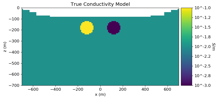
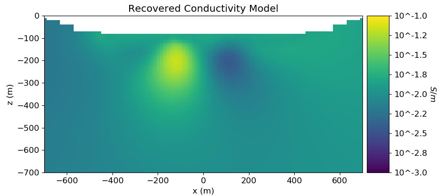
Plotting True and Recovered Conductivity Model

# Load true conductivity model
true_conductivity_model = np.loadtxt(str(true_conductivity_filename))
true_conductivity_model_log10 = np.log10(true_conductivity_model[ind_active])

# Plot True Model
fig = plt.figure(figsize=(9, 4))

plotting_map = maps.ActiveCells(mesh, ind_active, np.nan)

ax1 = fig.add_axes([0.1, 0.12, 0.72, 0.8])
mesh.plotImage(
    plotting_map * true_conductivity_model_log10,
    ax=ax1,
    grid=False,
    clim=(np.min(true_conductivity_model_log10), np.max(true_conductivity_model_log10)),
    range_x=[-700, 700],
    range_y=[-700, 0],
    pcolorOpts={"cmap": "viridis"},
)
ax1.set_title("True Conductivity Model")
ax1.set_xlabel("x (m)")
ax1.set_ylabel("z (m)")

ax2 = fig.add_axes([0.83, 0.12, 0.05, 0.8])
norm = mpl.colors.Normalize(
    vmin=np.min(true_conductivity_model_log10),
    vmax=np.max(true_conductivity_model_log10),
)
cbar = mpl.colorbar.ColorbarBase(
    ax2, norm=norm, orientation="vertical", cmap=mpl.cm.viridis, format="10^%.1f"
)

cbar.set_label("$S/m$", rotation=270, labelpad=15, size=12)

plt.show()

# Plot Recovered Model
fig = plt.figure(figsize=(9, 4))

# Make conductivities in log10
recovered_conductivity_model_log10 = np.log10(np.exp(recovered_conductivity_model))

ax1 = fig.add_axes([0.1, 0.12, 0.72, 0.8])
mesh.plotImage(
    plotting_map * recovered_conductivity_model_log10,
    normal="Y",
    ax=ax1,
    grid=False,
    clim=(np.min(true_conductivity_model_log10), np.max(true_conductivity_model_log10)),
    range_x=[-700, 700],
    range_y=[-700, 0],
    pcolorOpts={"cmap": "viridis"},
)
ax1.set_title("Recovered Conductivity Model")
ax1.set_xlabel("x (m)")
ax1.set_ylabel("z (m)")

ax2 = fig.add_axes([0.83, 0.12, 0.05, 0.8])
norm = mpl.colors.Normalize(
    vmin=np.min(true_conductivity_model_log10),
    vmax=np.max(true_conductivity_model_log10),
)
cbar = mpl.colorbar.ColorbarBase(
    ax2, norm=norm, orientation="vertical", cmap=mpl.cm.viridis, format="10^%.1f"
)
cbar.set_label("$S/m$", rotation=270, labelpad=15, size=12)

plt.show()

• 
• 

Out:

/Users/josephcapriotti/codes/simpeg/tutorials/05-dcr/plot_inv_2_dcr2d.py:381: UserWarning: Matplotlib is currently using agg, which is a non-GUI backend, so cannot show the figure.
  plt.show()
/Users/josephcapriotti/codes/simpeg/tutorials/05-dcr/plot_inv_2_dcr2d.py:414: UserWarning: Matplotlib is currently using agg, which is a non-GUI backend, so cannot show the figure.
  plt.show()

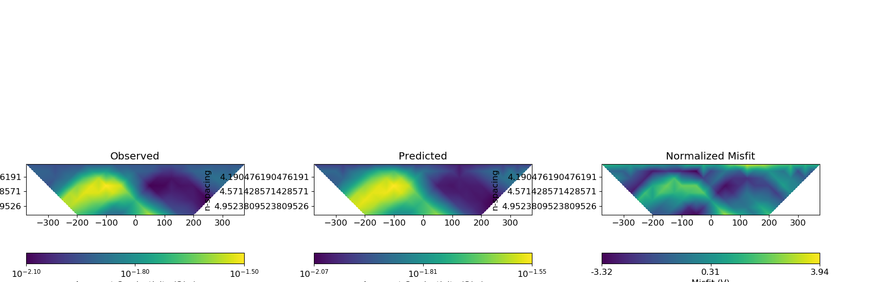
Plotting Predicted DC Data and Misfit

# Predicted data from recovered model
dpred = inv_prob.dpred
dc_data_predicted = data.Data(survey, dobs=dpred)

data_array = [dc_data, dc_data_predicted, dc_data]
dobs_array = [None, None, (dobs - dpred) / std]

fig = plt.figure(figsize=(17, 5.5))
plot_title = ["Observed", "Predicted", "Normalized Misfit"]
plot_type = ["appConductivity", "appConductivity", "misfitMap"]
plot_units = ["S/m", "S/m", ""]
scale = ["log", "log", "linear"]

ax1 = 3 * [None]
norm = 3 * [None]
cbar = 3 * [None]
cplot = 3 * [None]

for ii in range(0, 3):

    ax1[ii] = fig.add_axes([0.33 * ii + 0.03, 0.05, 0.25, 0.9])
    cplot[ii] = plot_pseudoSection(
        data_array[ii],
        dobs=dobs_array[ii],
        ax=ax1[ii],
        survey_type="dipole-dipole",
        data_type=plot_type[ii],
        scale=scale[ii],
        space_type="half-space",
        pcolorOpts={"cmap": "viridis"},
    )
    ax1[ii].set_title(plot_title[ii])

plt.show()

Out:

/Users/josephcapriotti/codes/simpeg/tutorials/05-dcr/plot_inv_2_dcr2d.py:454: UserWarning: Matplotlib is currently using agg, which is a non-GUI backend, so cannot show the figure.
  plt.show()